
Causal Explainability
Most explanation methods describe how a model's output depends on its inputs; causal explainability asks how outcomes would change under interventions in the world, which needs an explicit causal model and separates direct, indirect and spurious sources of disparity.
Overview
Chapters 73 and 74 presented explanations that describe a model: how much each input moved the output, and which change of inputs would have changed the decision. Such explanations are often read as if they described the world: income "drives" the credit decision, a higher balance "would" get the loan approved, ethnic origin "has no effect" because its attribution is zero. These readings are causal claims about the decision subject's situation, and they are justified only under causal assumptions that the explanation methods do not state.
Causal explainability makes those assumptions explicit. It uses the language of structural causal models (Chapter 30) to ask what would happen to an outcome, or to a model's decision, if some variable were set to a different value by an intervention, taking into account everything that variable affects. This matters for fairness in three ways. It determines whether an explanation can safely be turned into advice, as Chapter 74 showed for recourse. It determines how credit is shared between a protected attribute and the features it influences, which an assessor needs in order to distinguish direct discrimination from effects that pass through other variables. And it allows an observed disparity to be decomposed into parts with different legal and normative significance.
The chapter first sets out the causal hierarchy and the two different targets an explanation can have. It then shows when standard model-agnostic tools have a causal reading, presents causal variants of Shapley values, introduces actual causation, necessity and sufficiency, and describes causal explanation of neural networks. The last main section turns to the causal explanation of disparities. The causal fairness criteria themselves are defined in Chapter 18 and developed in Chapters 30 to 33; this chapter concerns explanation.
Learning objectives:
- Distinguish explaining a model's input and output behavior from explaining how outcomes depend on features in the world, and place each on the causal hierarchy.
- State the conditions under which a partial dependence plot estimates a causal effect.
- Define marginal, conditional, causal and asymmetric Shapley values and explain how each assigns credit when features are causally related.
- Explain actual causation, necessity and sufficiency as foundations for explanation and how explanation scores quantify them.
- Describe causal approaches to explaining neural networks, including causal mediation analysis of bias.
- Apply the causal explanation formula to decompose a disparity into direct, indirect and spurious components.
Key questions
- When can an explanation of a model be read as an explanation of why an outcome occurred or what would change it?
- How should credit be shared between a variable and the variables it causes?
- What makes one factor, rather than another, the cause of a decision?
- Through which pathways does a protected attribute affect a decision, and how much of an observed disparity flows through each?
- How much causal knowledge does each kind of causal explanation require, and what happens when that knowledge is wrong?
Definitions and terminology
Structural causal model (SCM). A set of variables, each determined by a function of its direct causes (parents) and an exogenous noise term, together with a distribution over the noise. Its graph is usually assumed acyclic (Chapter 30).
Intervention. An operation, written do(X = x), that sets X to x by replacing its structural equation, so that X no longer responds to its usual causes while its effects respond to the new value (Pearl, 2009).
Causal hierarchy. The classification of questions by Pearl (2019) into three levels: association (what does observing X tell me about Y?), intervention (what happens to Y if I set X?) and counterfactuals (what would have happened to Y had X been different, given what actually happened?). A question at a level can be answered only with information from that level or a higher one.
Direct, indirect and spurious effect. The direct effect of A on Y is transmitted along the edge A → Y; an indirect effect is transmitted through mediators (A → W → Y); a spurious association arises from paths that are not causal from A, for example through a common cause Z of A and Y (A ← Z → Y) (Zhang and Bareinboim, 2018).
Back-door criterion. A graphical condition under which adjusting for a set of variables XC identifies the causal effect of XS on Y: no variable in XC is a descendant of XS, and XC blocks every path between XS and Y that contains an arrow into XS (Zhao and Hastie, 2021).
Actual cause. A particular event that caused a particular outcome in a specific situation, as opposed to a general causal tendency. Halpern and Pearl (2005a) define it using structural equations and counterfactuals.
Necessity and sufficiency. A factor is necessary for an outcome if, had it been absent, the outcome would not have occurred; sufficient if its presence would produce the outcome. Probabilistic versions measure how likely each is (Galhotra, Pradhan and Salimi, 2021; Watson et al., 2021).
Mediator. A variable on a causal path between a cause and an effect. In causal mediation analysis of a neural network, internal components such as neurons or attention heads are treated as mediators between input and output (Vig et al., 2020).
Two targets of explanation
Explaining the model and explaining the world
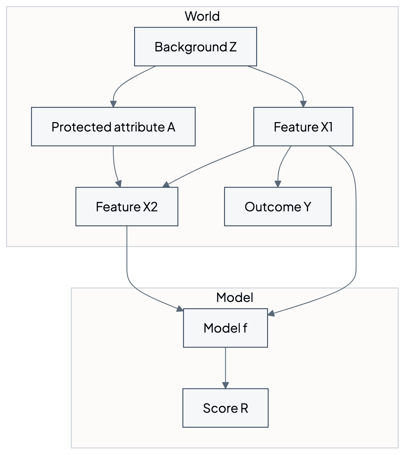
An explanation can have two different targets. The first is the model: the function f that maps inputs to outputs. Questions about the model are always causal in a narrow sense, because the inputs of a model causally determine its output and the assessor can intervene on them freely: feed in a changed input and observe the changed output. Janzing, Minorics and Blöbaum (2020) build on this point when they argue that dropping a feature in an attribution should be modeled as an intervention on the model's input, which leads to marginal (interventional) rather than conditional expectations (Chapter 73).
The second target is the world: the data-generating process in which features, protected attributes and outcomes are causally connected. Questions about the world ask how the outcome Y, or the decision a person would receive, depends on a feature when that feature is changed in reality, with all its consequences. A model's explanation answers such questions only if the model and its explanation are combined with a causal model of the world.
Zhao and Hastie (2021), following earlier work they cite, distinguish three notions of variable importance: the effect of a variable on the fitted function taken at face value; its contribution to predictive accuracy; and its causal effect, the change in the outcome if one could intervene on the variable. Only the third, they observe, is about the science rather than about the prediction.
Source: validant.ai.
An attribution to X2 in this diagram can describe how much f depends on X2 (the model target). Whether X2 matters for the person's outcome Y, or whether part of X2's attribution should be credited to A or to X1 because they cause X2, are questions about the world target and need the left-hand side of the diagram.
The causal hierarchy and explanation methods
Pearl (2019) places most of current machine learning at the first level of the causal hierarchy, association, because it fits functions to observed data. Interventional questions, such as what happens if the price is doubled, cannot in general be answered from data collected without that intervention, and counterfactual questions, such as what would have happened had one acted differently, require retrospective reasoning about a specific situation and sit at the top. Counterfactuals subsume the lower levels: a model that answers counterfactual queries can also answer interventional and associational ones.
Explanation methods can be located on the same hierarchy. Permutation importance and conditional Shapley values summarize associations between features and the model's output in the data. Integrated gradients and interventional Shapley values intervene on the model's inputs, which is an intervention on the model but not on the world. Causal Shapley values and recourse through minimal interventions (Chapter 74) intervene on variables of a causal model of the world. Counterfactual explanations in the sense of Wachter et al. (2018) use the language of counterfactuals but, without a structural model, they compute nearby points rather than structural counterfactuals; Karimi, Schölkopf and Valera (2021) show what changes when the counterfactual is computed in a structural model.
Causal readings of model-agnostic tools
When a partial dependence plot is causal
The partial dependence plot (Chapter 73) of a feature set XS averages the model's prediction over the observed distribution of the remaining features XC while XS is held at a value xS:
Zhao and Hastie (2021) observe that this has exactly the same form as Pearl's back-door adjustment formula, which expresses the expected outcome under the intervention do(XS = xS) as an average of E[Y | xS, xC] over the marginal distribution of XC. When the model g approximates E[Y | X] well and XC satisfies the back-door criterion with respect to XS and Y, the partial dependence plot therefore estimates the causal effect of XS on Y.
They state three requirements for causal interpretation of a black-box model: a model with good predictive performance, domain knowledge in the form of a causal diagram, and suitable visualization tools. The back-door criterion has two parts: no variable in XC may be a descendant of XS, and XC must block every back-door path between XS and Y. Heuristically, every back-door path corresponds to a common cause of XS and Y, and all of them, including unmeasured confounders, must be adjusted for.
The conditions fail in typical fairness applications. If a model includes features that are descendants of the feature of interest, such as a credit history that is shaped by income, the first condition fails. If important confounders are not among the model's inputs, the second fails. A partial dependence plot of a model trained on observational lending data is therefore usually a description of the model, not an estimate of what a change in income would do to repayment.
Causal Shapley values
How the value function encodes causal assumptions
Chapter 73 showed that Shapley-based attributions depend on how absent features are represented. Heskes, Sijben, Bucur and Claassen (2020) make the causal content of that choice explicit by defining the value of a coalition S as the expected prediction under an intervention that sets the features in S to their observed values:
The distribution of the absent features is then P(XS̄ | do(XS = xS)), which depends on the causal graph. Replacing it with P(XS̄ | xS) gives conditional Shapley values; when the intervention is taken to be on the model's inputs, so that the absent features keep their marginal distribution, the definition reduces to marginal Shapley values. Heskes et al. (2020) show that these causal Shapley values can be derived for general causal graphs using Pearl's do-calculus without losing the Shapley properties, and that they allow each feature's contribution to be decomposed into a direct effect, the change in prediction caused by the feature itself, and an indirect effect, the change caused by the shift that intervening on it induces in the distribution of other features. Marginal Shapley values, by construction, represent direct effects only, so that root causes with strong indirect effects can be ignored entirely.
Frye, Rowat and Feige (2020) take a different route. Symmetric Shapley values average a feature's marginal contribution over all orderings of the features. Asymmetric Shapley values relax the symmetry axiom and average over a distribution w(π) of orderings chosen to respect causal knowledge:
In the distal approach, w puts weight only on orderings in which known causal ancestors come before their descendants, so that ancestors are credited with their effect while descendants are still unknown and descendants receive only their incremental effect. In the proximate approach, the orderings are anti-causal and credit goes first to immediate causes. With no causal knowledge, both reduce to the uniform weighting of symmetric Shapley values (Frye et al., 2020).
Wang, Wiens and Lundberg (2021) argue that attributing credit to nodes cannot explain the whole causal graph and propose Shapley Flow, which assigns credit to the edges of the graph instead. They show that it is the unique solution to a generalization of the Shapley axioms to directed acyclic graphs, and that the edge-based view lets users see how importance flows through a system and reason about interventions.
Worked example: season, temperature and bike rentals
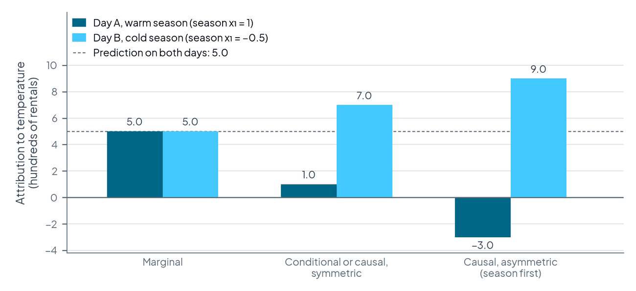
Heskes et al. (2020) illustrate the differences with a causal chain in which X1 is the season, X2 the temperature and the prediction is bike rental. Suppose, with invented numbers, that both features are standardized to mean 0, that E[X2 | x1] = 0.8 x1, and that a trained model happens to use only temperature: f(x1, x2) = 10 x2, measured in hundreds of rentals relative to average, so the base value is 0. Consider two days with the same temperature x2 = 0.5: day A in the warm season (x1 = 1), day B in the cold season (x1 = −0.5). The model predicts 5.0 on both days.
For the two-feature game the Shapley values follow directly from v(∅), v({1}), v({2}) and v({1, 2}) = 5. Marginal Shapley values set v({1}) = 0, because the model ignores season and season is not allowed to shift temperature. Conditional and causal Shapley values in the chain set v({1}) = 10 · 0.8 · x1, because knowing (or setting) the season changes the expected temperature. Asymmetric Shapley values with the distal ordering credit season first, with its full effect on expected temperature, and give temperature only its deviation from what the season implies.
| Value function | Day A: season | Day A: temperature | Day B: season | Day B: temperature |
|---|---|---|---|---|
| Marginal | 0.0 | 5.0 | 0.0 | 5.0 |
| Conditional or causal, symmetric | 4.0 | 1.0 | −2.0 | 7.0 |
| Causal, asymmetric (season first) | 8.0 | −3.0 | −4.0 | 9.0 |
Source: computed for this chapter following the patterns described by Heskes et al. (2020); every row sums to the prediction of 5.0.
Source: validant.ai.
The marginal explanation is identical on both days, although the same temperature is lower than normal for the warm season and higher than normal for the cold one; Heskes et al. (2020) use exactly this observation to argue that marginal Shapley values embody a counterintuitive notion of what is "normal". The asymmetric explanation says that on day A the season would have predicted 8.0 and the cool weather cost 3.0, while on day B the cold season would have predicted −4.0 and the mild weather added 9.0. If the arrow were reversed, so that temperature causes X1 (the structure Heskes et al. call a fork, because temperature then causes both X1 and the outcome), causal Shapley values would give X1 nothing, because intervening on it would not change temperature, while symmetric conditional Shapley values would still give it credit: Heskes et al. (2020) note that symmetric conditional Shapley values do not distinguish between any of the causal structures they compare (chain, fork, confounder and cycle).
The fairness reading is direct. Replace season by a protected attribute and temperature by a feature it influences, such as a neighborhood indicator. Marginal Shapley values give the protected attribute zero whenever the model does not read it; asymmetric Shapley values with the attribute first credit it with everything it does to the prediction through the features it causes. The second reading is what an assessor needs to see how much of a prediction a protected attribute is responsible for; the first is what is needed to see which inputs the model uses. Both are correct answers to different questions.
Unresolved discrimination with asymmetric Shapley values
Frye et al. (2020) use asymmetric Shapley values to measure unresolved discrimination (Kilbertus et al., 2017; Chapter 18): the influence of a sensitive attribute on a model's output through pathways that are not mediated by designated resolving variables. Their example is college admissions, in which gender should not influence admission directly, but genders may apply to departments at different rates and departments differ in competitiveness, so department choice is a resolving variable. They use a variant of the proximate approach that weights only orderings in which all resolving variables come before all sensitive attributes:
with R the resolving variables and S the sensitive attributes. The resulting value for a sensitive attribute is its incremental effect after the resolving variables have been accounted for, which is the influence the designation treats as unfair.
Actual causation, necessity and sufficiency
What makes something the cause
Attribution methods distribute credit; they do not say whether a particular factor was the cause of a particular decision. Halpern and Pearl (2005a) give a definition of actual causation in structural models. Informally, X = x is an actual cause of an outcome φ in a given situation if three conditions hold. First (AC1), both X = x and φ actually occur. Second (AC2), the variables can be split into those on the causal process from X to φ and the rest, such that (a) for some alternative setting of X and some setting of the remaining variables, φ would not have occurred, and (b) with X at its actual value and the remaining variables at that same setting, φ still occurs even if any of the variables on the causal process are reset to their actual values. Third (AC3), X is minimal: no part of it satisfies the first two conditions.
The definition is designed to handle cases that defeat simple counterfactual dependence, such as the example of two fires advancing on a house, where fire A burned the house first although fire B would have burned it anyway. Halpern and Pearl (2005b) build an account of explanation on this definition.
Beckers (2022) connects these notions to explainable AI. Because machine learning models are increasingly used to predict the results of actions, an explanation that is to be reliably action-guiding must be causal. He formally defines sufficient explanations, which say under which conditions an action guarantees a particular output, and counterfactual explanations, which say which change of an observed input would produce a change in an already observed output, and offers a definition of actual causation founded on action-guiding explanations, under which an actual cause is part of a good sufficient explanation for which there exist counterfactual values that would not have made the explanation better. He also shows how actual causation can be used to refine path-specific notions of fairness.
Probabilistic necessity and sufficiency
Watson et al. (2021) argue that necessity and sufficiency are the building blocks of all successful explanations, yet have been conceptually underdeveloped and inconsistently applied in explainable artificial intelligence. They provide a formal framework that unifies seemingly disparate local explanation methods, such as feature attributions, rule lists and counterfactuals, in terms of necessity and sufficiency, and a sound and complete algorithm for computing explanatory factors with respect to a given context.
Galhotra, Pradhan and Salimi (2021) define explanation scores for a black-box decision algorithm f embedded in a probabilistic causal model. For an attribute X with values x and baseline x′, decision o (favorable) and o′ (unfavorable), and a context K = k, the necessity score is the probability that the decision would have been unfavorable had X been x′, among cases where X = x and the decision was favorable; the sufficiency score is the probability that the decision would have been favorable had X been x, among cases where X = x′ and the decision was unfavorable:
Their system, LEWIS, uses these scores to rank attributes for an individual (for a rejected applicant, how likely a different value of an attribute would have led to approval), to describe an algorithm's global behavior, and to recommend minimal causal interventions on actionable attributes that are sufficient, with high probability, to change a future decision. The scores are counterfactual quantities, at the top of the causal hierarchy, and they require either a causal model or assumptions under which they can be bounded or estimated from data.
Attributions and counterfactuals as complementary
Kommiya Mothilal, Mahajan, Tan and Sharma (2021) interpret feature attributions and counterfactual explanations within the actual causality framework. They show how to derive feature attributions from a set of counterfactual examples, which convey whether a subset of features is necessary or sufficient for changing the outcome, information that attribution methods cannot provide, and how counterfactual examples can be used to evaluate attribution explanations in terms of necessity and sufficiency. On three benchmark data sets (Adult-Income, LendingClub and German-Credit) they find that LIME and SHAP on the one hand and the counterfactual methods of Wachter et al. and DiCE on the other often disagree on feature importance rankings, which they interpret as evidence that the two families answer complementary questions.
| Method | Question answered | Causal knowledge needed | Output |
|---|---|---|---|
| Partial dependence (causal reading) | Effect of setting a feature on Y | Graph satisfying back-door | Curve |
| Causal Shapley values | Credit under interventions | Causal graph or chain graph | Attribution per feature |
| Asymmetric Shapley values | Credit respecting causal order | Partial causal ordering | Attribution per feature |
| Shapley Flow | Credit along causal edges | Full causal graph | Attribution per edge |
| Necessity and sufficiency scores | Would the decision differ? | Probabilistic causal model | Probability per attribute |
| Causal explanation formula | Sources of a disparity | Standard fairness model | Direct, indirect, spurious |
Causal explanation inside neural networks
Attribution as average causal effect
Chattopadhyay, Manupriya, Sarkar and Balasubramanian (2019) view a neural network architecture as a structural causal model and propose an attribution method based on the average causal effect of an input neuron on an output neuron, computed by intervening on the input and taking interventional expectations of the output, with algorithms that make the computation efficient for high-dimensional inputs and recurrent networks. The approach makes explicit that attribution is, in their words, an inherently causal question about the effect of an input on the prediction function.
Schwab and Karlen (2019) frame explanation as a causal learning task and train a separate explanation model, CXPlain, to estimate how much each input causes the output of the explained model. Their causal objective follows Granger's definition, under which an input causes an output if the output is better predicted with that input than without it; the two assumptions of Granger causality (all relevant variables are included, and causes precede effects) hold by construction for a model's inputs and outputs. CXPlain uses bootstrap ensembling to quantify the uncertainty of its importance estimates. Both methods are causal with respect to the model, the first target of explanation, not with respect to the world.
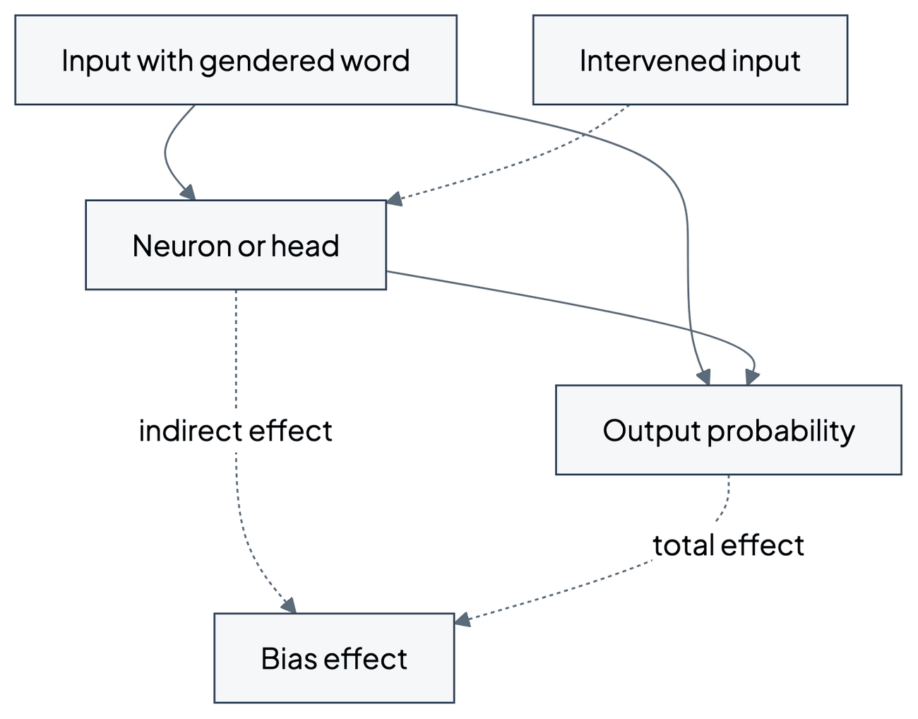
Causal mediation analysis of bias
Vig et al. (2020) apply causal mediation analysis to pre-trained Transformer language models, treating individual neurons and attention heads as mediators between an input (a sentence) and the model's output, and intervening on inputs and on internal components to measure how much of an effect flows through each. In a case study of gender bias, using three data sets designed to measure a model's sensitivity to grammatical gender, they find that gender bias effects are sparse (concentrated in a small part of the network), synergistic (amplified or repressed by different components) and decomposable into effects flowing directly from the input and indirectly through the mediators. Mediation analysis of this kind locates where in a model a biased behavior is produced, which is a precondition for targeted interventions on large models (Chapters 67 and 80).
Source: validant.ai.
Causal explanation of disparities
The causal explanation formula
Fairness assessments start from observed disparities. Zhang and Bareinboim (2018) ask how an observed disparity can be explained by the causal mechanisms that produce it. In their standard fairness model, X is the protected attribute (written A in this compendium), Y the outcome or decision, W mediators on causal paths from A to Y, and Z confounders that are associated with A and also affect Y. They distinguish three mechanisms: direct discrimination along A → Y; indirect discrimination along causal paths through mediators, A → W → Y; and spurious discrimination along non-causal paths, such as the back-door path A ← Z → Y.
The observed disparity is measured by the total variation, which is the demographic parity difference of Chapter 14 written for an outcome y:
They define counterfactual direct (Ctf-DE), indirect (Ctf-IE) and spurious (Ctf-SE) effects in non-parametric structural causal models and prove the causal explanation formula, which relates them to the total variation for any functional form of the structural equations and any distribution of the exogenous variables:
In words, the disparity experienced by those who have the attribute value a1, relative to a0, equals the disparity due to spurious association, plus the effect of indirect mechanisms, minus the advantage the group would have gained in the absence of direct discrimination, with the direct effect measured in the reverse direction. A second form expresses the total variation in terms of the direct effect from a0 to a1 minus reverse spurious and indirect effects.
In linear structural models the formula takes the intuitive additive form
and Zhang and Bareinboim (2018) show how each term can be estimated from observational data with partial regression coefficients under the assumptions of the linear standard model. They also show that measures such as the total variation cannot by themselves distinguish the three mechanisms.
Worked example: decomposing a disparity
Consider an invented linear version of the standard fairness model for a continuous credit outcome Y (for example an offered credit limit in standardized units; for a continuous outcome the total variation is the difference in group means). A background variable Z (for example regional economic conditions) is standard normal; the protected attribute A equals 1 when Z plus independent standard normal noise is positive, so that A and Z are correlated; a mediator W (for example the recorded debt ratio, inverted so that higher is better) follows W = 0.5A + 0.4Z + noise; and the outcome follows Y = 0.10A + 0.30W + 0.20Z + noise. A therefore affects Y directly (coefficient 0.10) and through W (0.5 · 0.30 = 0.15), and A and Y share the common cause Z.
The three effects in this linear model are:
- Direct effect: 0.10, the change in Y from switching A with W and Z held at their natural values.
- Indirect effect: 0.30 · 0.5 = 0.15, the change transmitted through the mediator.
- Spurious effect: (0.20 + 0.30 · 0.4) times the difference in the mean of Z between the groups. With Z and the noise both standard normal, E[Z | A = 1] − E[Z | A = 0] = 2/√π ≈ 1.128, so the spurious effect is 0.32 · 1.128 ≈ 0.361.
The total variation is therefore 0.10 + 0.15 + 0.361 ≈ 0.611. A simulation with 400,000 draws (NumPy default_rng, seed 5) gives an observed gap in mean outcomes of 0.606 and a measured difference in mean Z of 1.128, with which the three components sum to 0.611; the observed gap matches the analytical value within sampling error.
| Component | Pathway | Value | Share of gap |
|---|---|---|---|
| Direct effect | A → Y | 0.100 | 16% |
| Indirect effect | A → W → Y | 0.150 | 25% |
| Spurious effect | A ← Z → Y and A ← Z → W → Y | 0.361 | 59% |
| Total variation | Observed gap | 0.611 | 100% |
Source: computed for this chapter; shares rounded.

Source: validant.ai.
The decomposition changes the assessment. A demographic parity analysis reports a gap of 0.611 and nothing else. The causal explanation says that about one sixth of it is direct, the component that corresponds most closely to direct discrimination (Chapter 23); a quarter flows through the mediator, whose legitimacy depends on whether the debt ratio is a justified criterion or itself carries past discrimination; and the largest part reflects the association between group membership and regional conditions, which a model owner may have no control over but which may still raise questions of indirect discrimination. Each part calls for a different remedy (Part V). The numbers are only as good as the causal model: if Z had a direct path to W that was omitted, or an unmeasured confounder linked W and Y, the shares would be wrong.
Relation to path-specific fairness
The causal explanation formula is closely related to the path-specific criteria of Chapter 18: designating some paths as fair and others as unfair corresponds to deciding which components of the decomposition are acceptable. Plečko and Bareinboim (2024) develop this program into a general causal toolkit for fairness analysis. Asymmetric Shapley values for unresolved discrimination (Frye et al., 2020) and the actual-causation account of path-specific fairness proposed by Beckers (2022) are related tools that attach the judgment to individual predictions rather than to population averages.
Competing interpretations and limitations
Which counterfactual is the right one?
The debate between Janzing et al. (2020) and Heskes et al. (2020) is not about mathematics but about the target of explanation. If the question is which inputs the model's function depends on, intervening on the model's inputs is the right operation, and marginal Shapley values are the answer; Janzing et al. (2020) conclude that conditional expectations are the wrong notion of dropping a feature for this purpose. If the question is how the prediction for a person depends on facts about that person's situation, including what one fact implies about others, the causal structure of the world matters, and causal Shapley values are the answer. An assessor should decide which question is being asked before choosing a method, and should not present an answer to one as an answer to the other.
Identification and model dependence
Causal explanations need causal models, and causal models are assumptions. The partial dependence plot is causal only under the back-door criterion; causal Shapley values need at least a partial causal ordering or chain graph; necessity and sufficiency scores and the non-parametric causal explanation formula need counterfactual quantities that are often not identifiable from observational data and must be bounded or estimated under further assumptions. Karimi et al. (2020) show for recourse that guarantees are impossible without the true structural equations; the same logic applies to causal explanations generally. Kumar et al. (2020) observe that the remedies for the problems of Shapley-based explanations themselves require causal reasoning, which shifts the burden to the causal model.
Asymmetry has a price
Asymmetric Shapley values give up the symmetry axiom to encode causal order. Heskes et al. (2020) show that asymmetric values are sensitive to the insertion of causal links of zero strength: in their example of a network that computes the XOR of two binary features, assuming an ordering between the features changes the asymmetric attributions abruptly although nothing in the data changes. They conclude that asymmetric causal Shapley values may be preferable when causality follows a clear temporal order, whereas symmetric ones are much less sensitive to model misspecification. Which credit assignment is preferable (root causes, proximate causes or an even split) is partly a normative question about how responsibility should be shared, not only a technical one.
Causal explanation of the model is not fairness
Methods that are causal with respect to the model, such as average causal effects of input neurons or Granger-causal importance, explain the model's mechanism precisely. They do not by themselves reveal whether that mechanism is fair, because fairness depends on how the model's inputs relate to protected attributes and outcomes in the world. Causal mediation analysis of bias is informative because it is combined with inputs designed to vary a protected characteristic, which links the model mechanism to a fairness question.
Common questions
Are SHAP values causal?
Interventional SHAP values are causal with respect to the model: they describe how the output responds when inputs are set to new values. They are not causal with respect to the world, because they ignore how features affect one another. Causal Shapley values (Heskes et al., 2020) and asymmetric Shapley values (Frye et al., 2020) add causal knowledge about the world.
When can a partial dependence plot be read as a causal effect?
When the model predicts the outcome well and the other features satisfy the back-door criterion for the feature of interest: none is a descendant of it, and together they block every back-door path to the outcome (Zhao and Hastie, 2021).
Why does the protected attribute get zero attribution under one method and a large attribution under another?
Because the methods answer different questions. Marginal attributions give zero to any variable the model does not read. Causal and asymmetric attributions credit the protected attribute with its effects through the features it causes. An assessment should report both and say which question each answers.
Can a disparity be split into fair and unfair parts?
Yes, given a causal model: the causal explanation formula decomposes the observed gap into direct, indirect and spurious effects (Zhang and Bareinboim, 2018). Which parts are unfair is a normative and legal decision, often made by designating resolving variables or fair pathways (Chapter 18).
What if the causal graph is uncertain?
Report the explanation under each plausible graph, bound the quantities that are not identified, and state which conclusions are robust. When no defensible causal model exists, use causal methods for sensitivity analysis and rely on observational fairness criteria for the main finding.
Is a counterfactual explanation the same as a causal counterfactual?
No. A counterfactual explanation in the sense of Chapter 74 finds a nearby input that the model treats differently. A causal counterfactual asks what would have happened to the same individual, under the same background conditions, had one variable been set differently with all its consequences, which requires a structural model (Karimi, Schölkopf and Valera, 2021).
Do causal methods work for large language models?
Causal mediation analysis has been applied to Transformer language models to locate the components that mediate gender bias (Vig et al., 2020). Such analyses explain the model's mechanism; linking them to fairness requires inputs designed around the protected characteristic.
Conclusions
Causal explainability separates two questions that ordinary explanation methods run together: how a model's output depends on its inputs, and how outcomes and decisions depend on features of the world. The first is always answerable by intervening on the model. The second requires a causal model of the data-generating process, and with one, explanations gain capabilities that matter for fairness: partial dependence plots that estimate causal effects under stated conditions, Shapley values that credit a protected attribute with its effects through the features it influences, necessity and sufficiency scores that say whether a factor made the difference, and a decomposition of observed disparities into direct, indirect and spurious parts.
The methodological conclusion is that causal explanations should be used where the question is causal, which in fairness assessment it often is, and that the causal model must be treated as part of the explanation: stated, defended with domain knowledge, and varied to show which conclusions survive alternative assumptions. Reporting causal and non-causal explanations side by side, with the question each answers, protects against the two typical errors: reading a description of a model as a fact about the world, and presenting a causal decomposition as if its assumptions were facts.
Open questions
- How can causal explanations be made robust to uncertainty about the causal graph, and how should the remaining uncertainty be communicated to non-specialists?
- Which credit-sharing rule (symmetric, distal or proximate) best fits the normative questions of non-discrimination law, and can the choice be justified rather than conventional?
- How can counterfactual explanation scores be estimated reliably from observational data when they are only partially identified?
- How can causal mediation analysis scale to the size of current foundation models and link internal mechanisms to fairness outcomes in deployed applications?
- How should the components of the causal explanation formula be mapped to legal categories of direct and indirect discrimination across jurisdictions?
References
- Beckers, S. (2022). Causal explanations and XAI. In Proceedings of the First Conference on Causal Learning and Reasoning (Proceedings of Machine Learning Research, Vol. 177, pp. 90 - 109). https://proceedings.mlr.press/v177/beckers22a.html
- Chattopadhyay, A., Manupriya, P., Sarkar, A., & Balasubramanian, V. N. (2019). Neural network attributions: A causal perspective. In Proceedings of the 36th International Conference on Machine Learning (Proceedings of Machine Learning Research, Vol. 97, pp. 981 - 990). https://proceedings.mlr.press/v97/chattopadhyay19a.html
- Frye, C., Rowat, C., & Feige, I. (2020). Asymmetric Shapley values: Incorporating causal knowledge into model-agnostic explainability. In Advances in Neural Information Processing Systems 33 (pp. 1229 - 1239). https://proceedings.neurips.cc/paper_files/paper/2020/hash/0d770c496aa3da6d2c3f2bd19e7b9d6b-Abstract.html
- Galhotra, S., Pradhan, R., & Salimi, B. (2021). Explaining black-box algorithms using probabilistic contrastive counterfactuals. In Proceedings of the 2021 International Conference on Management of Data (pp. 577 - 590). https://doi.org/10.1145/3448016.3458455
- Halpern, J. Y., & Pearl, J. (2005a). Causes and explanations: A structural-model approach. Part I: Causes. The British Journal for the Philosophy of Science, 56(4), 843 - 887. https://doi.org/10.1093/bjps/axi147
- Halpern, J. Y., & Pearl, J. (2005b). Causes and explanations: A structural-model approach. Part II: Explanations. The British Journal for the Philosophy of Science, 56(4), 889 - 911. https://doi.org/10.1093/bjps/axi148
- Heskes, T., Sijben, E., Bucur, I. G., & Claassen, T. (2020). Causal Shapley values: Exploiting causal knowledge to explain individual predictions of complex models. In Advances in Neural Information Processing Systems 33 (pp. 4778 - 4789). https://proceedings.neurips.cc/paper_files/paper/2020/hash/32e54441e6382a7fbacbbbaf3c450059-Abstract.html
- Janzing, D., Minorics, L., & Blöbaum, P. (2020). Feature relevance quantification in explainable AI: A causal problem. In Proceedings of the Twenty Third International Conference on Artificial Intelligence and Statistics (Proceedings of Machine Learning Research, Vol. 108, pp. 2907 - 2916). https://proceedings.mlr.press/v108/janzing20a.html
- Karimi, A.-H., Schölkopf, B., & Valera, I. (2021). Algorithmic recourse: From counterfactual explanations to interventions. In Proceedings of the 2021 ACM Conference on Fairness, Accountability, and Transparency (pp. 353 - 362). https://doi.org/10.1145/3442188.3445899
- Karimi, A.-H., von Kügelgen, J., Schölkopf, B., & Valera, I. (2020). Algorithmic recourse under imperfect causal knowledge: A probabilistic approach. In Advances in Neural Information Processing Systems 33 (pp. 265 - 277). https://proceedings.neurips.cc/paper_files/paper/2020/hash/02a3c7fb3f489288ae6942498498db20-Abstract.html
- Kilbertus, N., Rojas-Carulla, M., Parascandolo, G., Hardt, M., Janzing, D., & Schölkopf, B. (2017). Avoiding discrimination through causal reasoning. In Advances in Neural Information Processing Systems 30. https://proceedings.neurips.cc/paper_files/paper/2017/hash/f5f8590cd58a54e94377e6ae2eded4d9-Abstract.html
- Kommiya Mothilal, R., Mahajan, D., Tan, C., & Sharma, A. (2021). Towards unifying feature attribution and counterfactual explanations: Different means to the same end. In Proceedings of the 2021 AAAI/ACM Conference on AI, Ethics, and Society (pp. 652 - 663). https://doi.org/10.1145/3461702.3462597
- Kumar, I. E., Venkatasubramanian, S., Scheidegger, C., & Friedler, S. (2020). Problems with Shapley-value-based explanations as feature importance measures. In Proceedings of the 37th International Conference on Machine Learning (Proceedings of Machine Learning Research, Vol. 119, pp. 5491 - 5500). https://proceedings.mlr.press/v119/kumar20e.html
- Pearl, J. (2009). Causality: Models, reasoning, and inference (2nd ed.). Cambridge University Press. https://doi.org/10.1017/CBO9780511803161
- Pearl, J. (2019). The seven tools of causal inference, with reflections on machine learning. Communications of the ACM, 62(3), 54 - 60. https://doi.org/10.1145/3241036
- Plečko, D., & Bareinboim, E. (2024). Causal fairness analysis: A causal toolkit for fair machine learning. Foundations and Trends in Machine Learning, 17(3), 304 - 589. https://doi.org/10.1561/2200000106
- Schwab, P., & Karlen, W. (2019). CXPlain: Causal explanations for model interpretation under uncertainty. In Advances in Neural Information Processing Systems 32. https://proceedings.neurips.cc/paper_files/paper/2019/hash/3ab6be46e1d6b21d59a3c3a0b9d0f6ef-Abstract.html
- Vig, J., Gehrmann, S., Belinkov, Y., Qian, S., Nevo, D., Sakenis, S., Huang, J., Singer, Y., & Shieber, S. (2020). Causal mediation analysis for interpreting neural NLP: The case of gender bias (arXiv:2004.12265). arXiv. https://arxiv.org/abs/2004.12265
- Wachter, S., Mittelstadt, B., & Russell, C. (2018). Counterfactual explanations without opening the black box: Automated decisions and the GDPR. Harvard Journal of Law & Technology, 31(2), 841 - 887. https://doi.org/10.2139/ssrn.3063289
- Wang, J., Wiens, J., & Lundberg, S. (2021). Shapley Flow: A graph-based approach to interpreting model predictions. In Proceedings of the 24th International Conference on Artificial Intelligence and Statistics (Proceedings of Machine Learning Research, Vol. 130, pp. 721 - 729). https://proceedings.mlr.press/v130/wang21b.html
- Watson, D. S., Gultchin, L., Taly, A., & Floridi, L. (2021). Local explanations via necessity and sufficiency: Unifying theory and practice. In Proceedings of the Thirty-Seventh Conference on Uncertainty in Artificial Intelligence (Proceedings of Machine Learning Research, Vol. 161, pp. 1382 - 1392). https://proceedings.mlr.press/v161/watson21a.html
- Zhang, J., & Bareinboim, E. (2018). Fairness in decision-making: The causal explanation formula. In Proceedings of the AAAI Conference on Artificial Intelligence, 32(1). https://doi.org/10.1609/aaai.v32i1.11564
- Zhao, Q., & Hastie, T. (2021). Causal interpretations of black-box models. Journal of Business & Economic Statistics, 39(1), 272 - 281. https://doi.org/10.1080/07350015.2019.1624293