
Threshold Optimization
Group-specific thresholds are the most direct post-processing route to equal opportunity, equalized odds or demographic parity; they need no retraining, but their cost, their need for randomization and their legal standing must be established case by case.
Overview
Post-processing interventions act after a model has been trained. They leave the training data and the learning algorithm untouched and change only how the model's output is turned into a decision. Among them, threshold optimization is the simplest and the most widely used: a score R is compared with a threshold, and the threshold is allowed to differ between groups so that a chosen fairness criterion is met. Because it needs only scores, outcomes and group membership on a held-out data set, the method applies to models that cannot be retrained, to purchased black-box models and to systems already in service, where a new model would need months of development and validation.
The idea rests on an observation that is easy to overlook. Applying one threshold to everyone looks neutral, but it implicitly assumes that the score has the same distribution and the same quality in every group. When either assumption fails, one shared threshold produces different selection rates and different error rates, even when the score is well calibrated within each group (Corbett-Davies et al., 2017). Group-specific thresholds correct the rates directly. They do not remove the underlying trade-offs between fairness criteria and between fairness and utility; they make those trade-offs explicit and quantifiable.
This chapter builds on the ROC view of separation in Chapter 15, where the convex-hull result of Hardt, Price and Srebro (2016) is outlined, and on the treatment of calibration in Chapter 16. It gives the operational detail: the optimization problems, the role of randomization, how thresholds are estimated and validated, how they can be deployed when the protected attribute may not be used at decision time, and where the law draws limits. Chapter 56 covers recalibration of the scores themselves, which is often a precondition for meaningful thresholds, and Chapter 57 covers more general transformations of predictions, including reject-option methods. The choice among pre-, in- and post-processing is the subject of Chapter 46.
Learning objectives:
- Formulate threshold optimization for demographic parity, equal opportunity and equalized odds as constrained utility maximization.
- Read group ROC curves to see which operating points a post-processing step can reach and why equalized odds may require randomization.
- Compute group-specific thresholds, their fairness effect and their utility cost on a worked example.
- Compare deployment with the protected attribute, with an estimate of it, and without it, and state the legal risks of each.
- Design a validation, monitoring and documentation plan for thresholds in production, including intersectional groups.
Key questions
- How can classification thresholds be adjusted after training so that a specific fairness criterion holds, without retraining or modifying the model?
- What are the mathematical relationships between threshold selection and the fairness criteria, and how should the trade-offs between them, and between fairness and utility, be navigated?
- When does a fairness criterion require randomized decisions, and is randomization acceptable in the application?
- What can be done when the protected attribute is unavailable at decision time, or may not lawfully be used?
- How stable are optimized thresholds once the population changes?
Definitions and terminology
Decision threshold. A value t such that the prediction is positive when the score reaches it: Ŷ = 1 if R ≥ t. In the compendium notation Y = 1 is the outcome the decision process looks for (for example, a loan is repaid), so a positive prediction is the favorable decision.
Group-specific threshold. A threshold ta that depends on the value a of the protected attribute A. The resulting classifier is Ŷ = 1 if R ≥ tA.
Operating point. The pair (FPRa, TPRa) that a decision rule produces in group a. Each threshold yields one operating point per group.
Group ROC curve. The curve of operating points traced by a threshold as it moves over all values, computed separately within each group (Chapter 15).
Derived predictor. A possibly randomized function of the score R and the protected attribute A alone (Hardt et al., 2016). Every threshold rule, with or without randomization, is a derived predictor. The features X play no further role once the score has been computed.
Randomized threshold. A rule that accepts everyone above an upper threshold, rejects everyone below a lower threshold and accepts with a fixed probability in between. It reaches operating points that lie on the straight line between two points of the ROC curve.
Post-processing. Any intervention that changes the mapping from model outputs to decisions after training, including threshold optimization, recalibration (Chapter 56) and prediction transformation (Chapter 57).
Leveling down. Meeting a parity criterion by worsening the outcomes or error rates of the better-served group without improving those of the worse-served group.
Fairness-utility frontier. The set of decision rules for which neither fairness (measured by a chosen disparity) nor utility can be improved without worsening the other. It is the Pareto frontier of the two objectives (Chapter 54).
Why a single threshold is not neutral
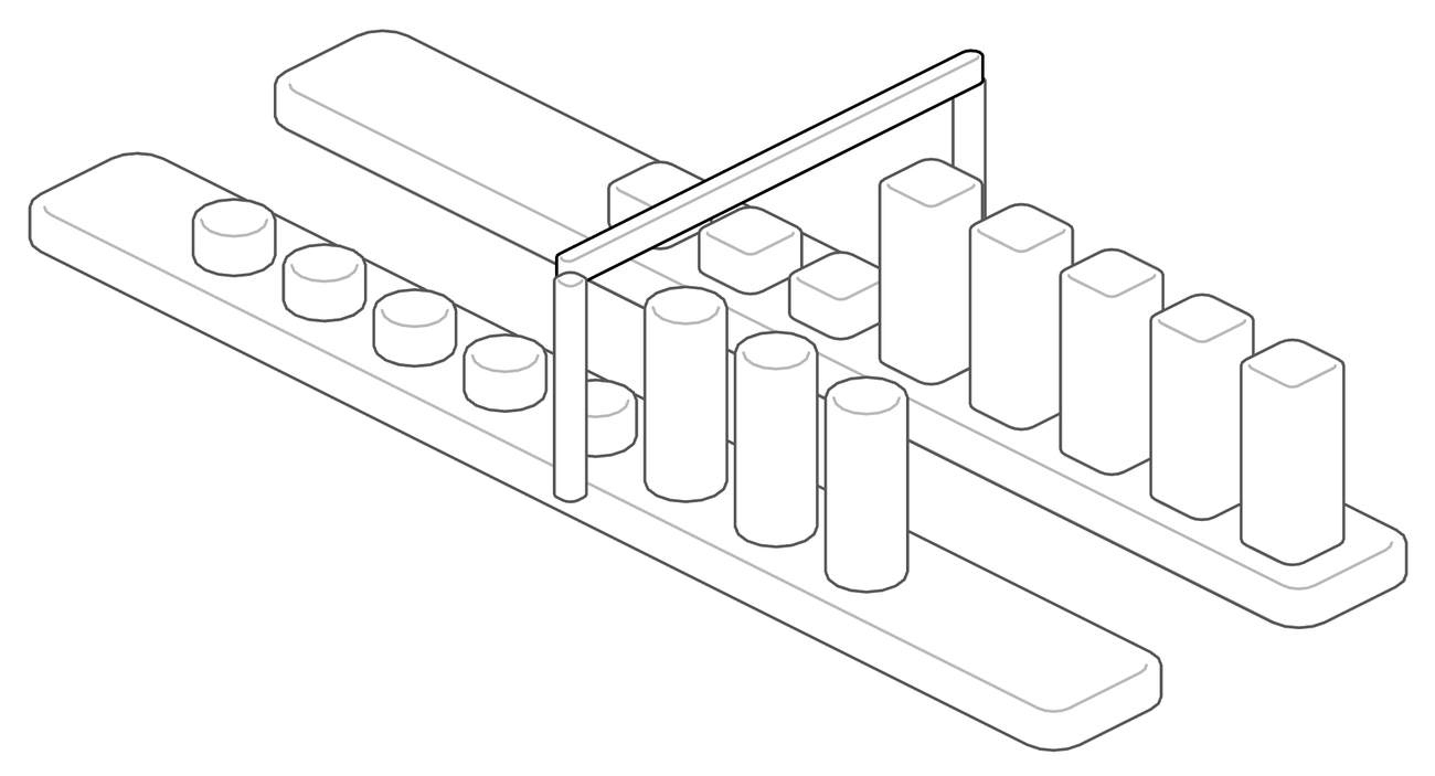
A score becomes a decision at a threshold. Common practice applies one threshold, often 0.5 for a predicted probability, to everyone. This rule treats all individuals with the same score alike, which is a meaningful kind of equal treatment. It does not, however, guarantee equal rates. Selection rates and error rates depend on how the scores are distributed in each group, and those distributions differ for two kinds of reasons.
Source: validant.ai.
The first reason is a difference in the outcome itself or in its predictors. If default is more common in one group in the training data, the score distribution of that group sits lower, and a common threshold selects fewer of its members. Corbett-Davies et al. (2017) state that a single decision threshold can, and generally does, result in racial disparities, and connect this to the problem of infra-marginality: when the tails of two risk distributions differ, a common cut produces different detention and false positive rates even when the score means the same in both groups. The second reason is a difference in score quality. If the features predict the outcome less well for one group, its ROC curve lies lower, and at any common threshold that group suffers more errors of at least one type. Hardt et al. (2016) emphasize, in their credit-score case study, that differences between group ROC curves indicate differences in prediction accuracy, not in the behavior of the people scored.
Either reason may itself reflect historical discrimination. In lending, past exclusion from credit leaves members of some groups with thinner credit files, which both lowers their scores and makes the scores less informative. Applying one threshold to such scores then denies credit to qualified applicants of the disadvantaged group more often than to others. Threshold optimization responds by letting the threshold vary with group membership, so that the chosen rate comparison comes out equal.
The same result shows why threshold optimization is the natural post-processing step. If any parity constraint is imposed on a decision maker with a good risk estimate, the best way to satisfy it is to move group thresholds, not to adopt some other rule. Lipton, Chouldechova and McAuley (2018) reach the parallel conclusion for impact parity: intervention through per-group thresholds maximizes accuracy subject to the parity constraint, and methods that try to avoid explicit group thresholds give suboptimal trade-offs.
The formal problems
Threshold rules and the three criteria
Let each group g ∈ {a, b} have its own threshold tg, so that the decision rule is
The three group criteria of Chapters 14 and 15 then become conditions on the thresholds. Demographic parity asks for equal selection rates:
Equal opportunity asks for equal true positive rates, that is, equal chances of a favorable decision among those with Y = 1:
Equalized odds adds equal false positive rates:
Each condition leaves many threshold pairs feasible. Demographic parity and equal opportunity each fix one degree of freedom, so a whole curve of threshold pairs satisfies them; equalized odds fixes two, and for deterministic thresholds it is usually infeasible except at trivial points. The choice among feasible pairs is made by utility.
Utility and loss
Hardt et al. (2016) express the objective as an expected loss E[ℓ(Ŷ, Y)], where ℓ assigns a cost to each pair of prediction and outcome. With no cost for correct decisions, the loss is determined by two numbers, the cost cFP of a false positive and the cost cFN of a false negative. Corbett-Davies et al. (2017) use the equivalent language of immediate utility: the expected benefit of the positive decisions minus a per-decision cost. In lending, the benefit is the margin earned on a repaid loan and the cost is the loss on a defaulted one.
For a well-calibrated score R = P(Y = 1 | X), the unconstrained optimal rule approves exactly when the expected gain of approval is positive. With gain g on a repaid loan and loss l on a defaulted one, the rule is
This is one threshold for everyone. Every fairness constraint is then a restriction on this problem, and its cost is the drop in expected utility relative to the unconstrained optimum.
Constrained optimization
The general problem is to maximize expected utility over the decision rules derived from (R, A) subject to the chosen criterion. Writing γa(Ŷ) = (FPRa, TPRa) for the operating point in group a, Hardt et al. (2016) state the equalized odds version as
For a binary score and a binary attribute this is a linear program in four variables, the probabilities of a positive decision for each combination of score value and group; its coefficients can be computed from the joint distribution of (Ŷ, A, Y), and its solution is the optimal equalized odds predictor derived from Ŷ and A (Hardt et al., 2016, Proposition 4.4). For a continuous score the feasible regions are not polytopes and the problem is no longer a linear program, but the authors show that it can be optimized efficiently by ternary search. With a score that takes finitely many values, as in the worked example below, the problem is again a linear program in the acceptance probabilities of each score value in each group.
Equal opportunity drops the false positive constraint. Assuming the group ROC curves are continuous, the optimal equal opportunity rule uses two deterministic thresholds, one per group, and is again found by a one-dimensional search over the common true positive rate (Hardt et al., 2016). Demographic parity is the simplest case: for any target selection rate, the threshold of each group is the corresponding quantile of its score distribution, and the optimal target is found by a search over a single number.
Relaxed constraints
Exact parity is rarely required in practice, and estimates from finite samples never show it exactly. A relaxed problem allows a disparity up to a tolerance ε, for example
Varying ε from zero to the disparity of the unconstrained rule traces the fairness-utility frontier. Corbett-Davies et al. (2017) show that threshold rules remain optimal when a constraint is required to hold only approximately, for example when false positive rates may differ by at most a constant δ across groups. Tolerances are supported in common tooling; the Fairlearn ThresholdOptimizer, for example, accepts a tolerance for demographic parity and rate-parity constraints but not for equalized odds (Fairlearn, n.d.-a).
Menon and Williamson (2018) give a general characterization: for cost-sensitive accuracy and fairness measures expressed as cost-sensitive risks, the Bayes optimal fairness-aware classifier is an instance-dependent thresholding of the class-probability function, and the size of the fairness-accuracy trade-off is determined by how closely the class probabilities for the target and for the sensitive feature are aligned. When the sensitive feature is an input, the instance-dependent correction reduces to a different constant threshold for each group.
The ROC geometry
What post-processing can reach
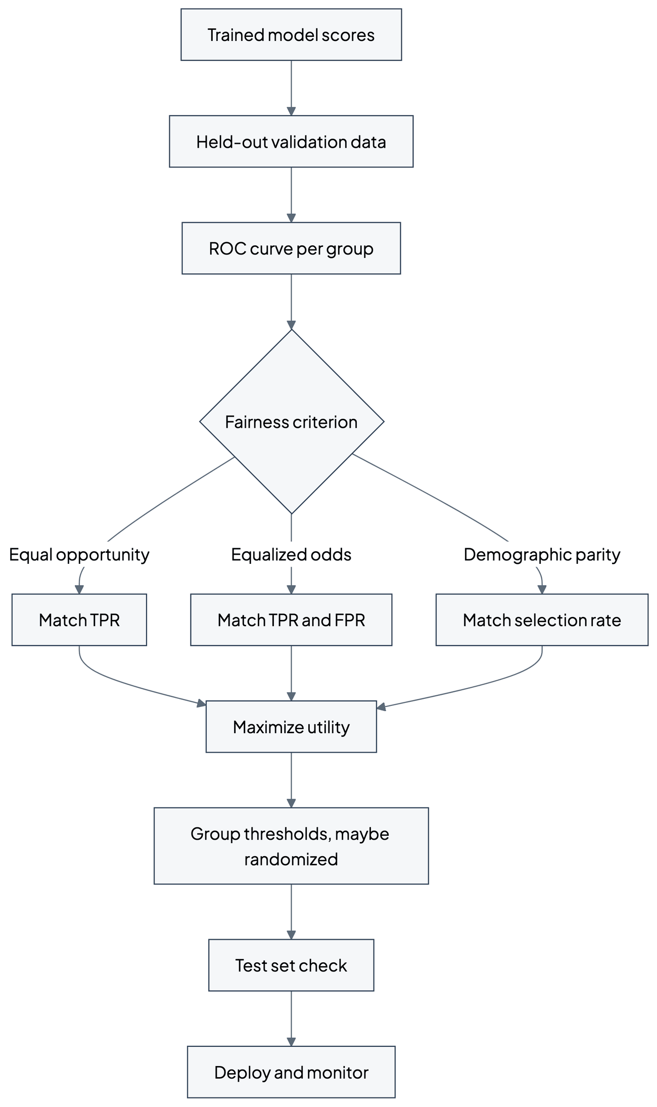
Plotting the group ROC curves in one plane shows every operating point a deterministic threshold can produce in each group. Randomization extends the reachable set: mixing two threshold rules yields any point on the straight segment joining their operating points, so the reachable region for group a is the convex hull of its ROC curve, including the corners (0, 0) and (1, 1). Only the upper-left boundary of this region matters for any sensible loss; points below the diagonal are worse than random guessing (Hardt et al., 2016).
The three criteria have a direct reading in this plane:
- Equal opportunity places the groups' operating points on one horizontal line (same TPR). Deterministic group thresholds can always achieve this when the curves are continuous.
- Equalized odds places the two operating points on the same point. Only points in the intersection of the reachable regions qualify. The optimal one lies on the upper-left boundary of that intersection, which is the pointwise minimum of the groups' ROC hulls (the upper concave envelopes of their ROC curves).
- Demographic parity is not a condition on the ROC plane alone. It constrains the selection rate pa·TPRa + (1 − pa)·FPRa, which mixes the two rates with the group base rate pa, so groups with different base rates end on different points.
Source: validant.ai.
Randomization and its meaning
A randomized threshold works as follows. For group a there are two thresholds, a lower ta and an upper t̄a, and an acceptance probability qa (written q rather than p to keep it apart from the base rate pa):
Hardt et al. (2016) use exactly this form in their FICO case study: above both thresholds people always qualify, and between them they qualify with some probability. Randomization is mathematically harmless, since the expected rates are what the criterion constrains, but it is often hard to defend. Two applicants with the same score and the same group can receive different decisions because of a coin flip. The Fairlearn documentation notes that a non-zero probability of a positive label for an individual is not acceptable in some application contexts (Fairlearn, n.d.-b). Randomization also matters when scores take only a few values: with a score in five bands, deterministic thresholds reach only five operating points per group, and even equal opportunity then generally needs a randomized acceptance probability at one band.
Leveling down
When one group's ROC curve lies everywhere below the other's, the intersection of the reachable regions is the region under the lower curve. The optimal equalized odds point therefore lies on the lower curve, and the better-served group must be moved to a point it could improve on, by deliberately adding noise to its decisions. Hardt et al. (2016) put it plainly: an equalized odds classifier must classify everyone as poorly as the hardest group, which in their FICO setting is why it cost more than twice as much as equal opportunity. The Fairlearn user guide names the same effect leveling down: better-off groups are worsened without making worse-off groups better off in absolute terms (Fairlearn, n.d.-b). Chapter 20 discusses why leveling down is a serious normative objection and not only a cost.
The same paper draws an incentive argument from this geometry. Under a maximum-profit rule, a small group that is poorly classified is treated poorly, because the decision maker has little reason to learn to classify it. Under equal opportunity, the cost of poor classification falls on the decision maker, who can respond by improving the score for that group; equalized odds gives a similar but much stronger incentive (Hardt et al., 2016).
Evidence from the credit-score case study
Hardt et al. (2016) apply the criteria to TransUnion TransRisk scores, with race as the protected attribute and the absence of a serious default as the favorable outcome, and model a lender for whom approving a borrower who defaults costs 82/18 times as much as rejecting one who would not. They compare five policies: maximum profit with a separate profit-maximizing threshold per group, a single race-blind threshold, demographic parity, equal opportunity and equalized odds. Under the maximum-profit and race-blind thresholds, Black applicants who would not default had a significantly harder time qualifying than others; under demographic parity the situation was reversed. At the 82 percent profitability point, the race-blind threshold earned 99.3 percent of the maximal profit, equal opportunity 92.8 percent, equalized odds 80.2 percent and demographic parity 69.8 percent, so equal opportunity cost less than a quarter of what demographic parity cost. The full table and its context are in Chapter 15.
Two lessons transfer. First, equalizing true positive rates required different thresholds for different groups, and equalized odds additionally required randomization. Second, within each group the equal opportunity threshold and the average equalized odds threshold lay between the maximum-profit threshold and the demographic parity threshold, so these criteria are intermediate interventions. The cost figures are specific to that data set and loss and are not general laws.
Worked example: thresholds for a lending score
This example is illustrative, with invented counts chosen so that every number can be recomputed. A lender's model outputs a repayment score R in five bands, and approves (Ŷ = 1) applicants whose score reaches a threshold. Y = 1 means the applicant repays. Group a has 1,000 applicants and group b has 500. The score is calibrated within each group: in every band the share of repayers equals the band value.
| Score band | Group a: repay / default | Group b: repay / default |
|---|---|---|
| 0.9 | 270 / 30 | 45 / 5 |
| 0.8 | 200 / 50 | 80 / 20 |
| 0.6 | 120 / 80 | 75 / 50 |
| 0.4 | 60 / 90 | 50 / 75 |
| 0.2 | 20 / 80 | 20 / 80 |
| Total | 670 / 330 | 270 / 230 |
Source: illustrative data constructed for this chapter.
The base rates are pa = 670/1,000 = 0.67 and pb = 270/500 = 0.54. The lender gains 1 unit on a repaid loan and loses 1 unit on a defaulted one, so the unconstrained rule approves when R ≥ 1/(1 + 1) = 0.5, that is, bands 0.6 and above. Because the score is calibrated in both groups, this single threshold is also the profit-maximizing threshold for each group separately.
Single threshold. In group a, it approves 120 + 200 + 270 = 590 of 670 repayers and 80 + 50 + 30 = 160 of 330 defaulters: TPRa = 0.881, FPRa = 0.485, selection rate 0.750. In group b, it approves 75 + 80 + 45 = 200 of 270 repayers and 50 + 20 + 5 = 75 of 230 defaulters: TPRb = 0.741, FPRb = 0.326, selection rate 0.550. Profit is 590 − 160 = 430 in group a and 200 − 75 = 125 in group b, 555 in total. A calibrated score and an identical rule thus leave qualified applicants of group b with a 14 percentage point lower chance of approval, which is the pattern Corbett-Davies et al. (2017) describe.
Optimal constrained rules. Solving the linear program over the acceptance probability of each band in each group, with acceptance required to be non-decreasing in the score, gives the following policies.
| Policy | Group a rule | Group b rule | TPR a / b | FPR a / b | Profit (share of max) |
|---|---|---|---|---|---|
| Single threshold | Bands ≥ 0.6 | Bands ≥ 0.6 | 0.881 / 0.741 | 0.485 / 0.326 | 555 (100%) |
| Demographic parity | Bands ≥ 0.6 | Bands ≥ 0.6, band 0.4 at 80% | 0.881 / 0.889 | 0.485 / 0.587 | 535 (96.4%) |
| Equal opportunity | Bands ≥ 0.6 | Bands ≥ 0.6, band 0.4 at 75.5% | 0.881 / 0.881 | 0.485 / 0.572 | 536.1 (96.6%) |
| Equalized odds | Band 0.9; band 0.8 at 87.9%; band 0.6 at 42.1% | Bands ≥ 0.6 | 0.741 / 0.741 | 0.326 / 0.326 | 513.7 (92.6%) |
Source: computed for this chapter by linear programming on the data in the previous table.
Several features of the general theory are visible. Equal opportunity is reached by lowering the threshold for group b into band 0.4. Since that band is coarse, exact equality needs a partial acceptance of 75.5 percent of band-0.4 applicants in group b; approving the whole band instead would give TPRb = 0.926 and overshoot the target, at a profit of 530. The extra approvals in group b are loans with a 40 percent repayment rate, so profit in group b falls from 125 to 106.1, a total cost of 3.4 percent. Demographic parity, reached here by raising group b's selection rate to 0.75, costs 3.6 percent; a different way of equalizing selection rates, raising group a's threshold to 0.8 so that both groups are selected at 0.55, is also feasible but earns only 515, which shows why the optimum is not simply "the same rate at any level".
Equalized odds behaves differently. Over the range of operating points that matters here, the group b ROC curve lies below the group a curve (it lies above it only at very low false positive rates, around group b's two highest bands), so the optimal common operating point is group b's own point (0.326, 0.741), and group a is moved down to it. Group a's applicants in band 0.8, who repay 80 percent of the time, are now approved only with probability 0.879, and those in band 0.6 with probability 0.421. Group b is untouched and gains nothing; group a's qualified applicants lose 14 percentage points of approval. This is leveling down in its plainest form, at a total cost of 7.4 percent. The group a rule in the table is one of many optimal ones: profit within a group is a linear function of that group's TPR and FPR alone (here 670·TPRa − 330·FPRa), so every rule that reaches the common point earns the same 388.7 in group a, and a solver may return any of them. The rule shown is the one that accepts band 0.9 in full.
Source: validant.ai.
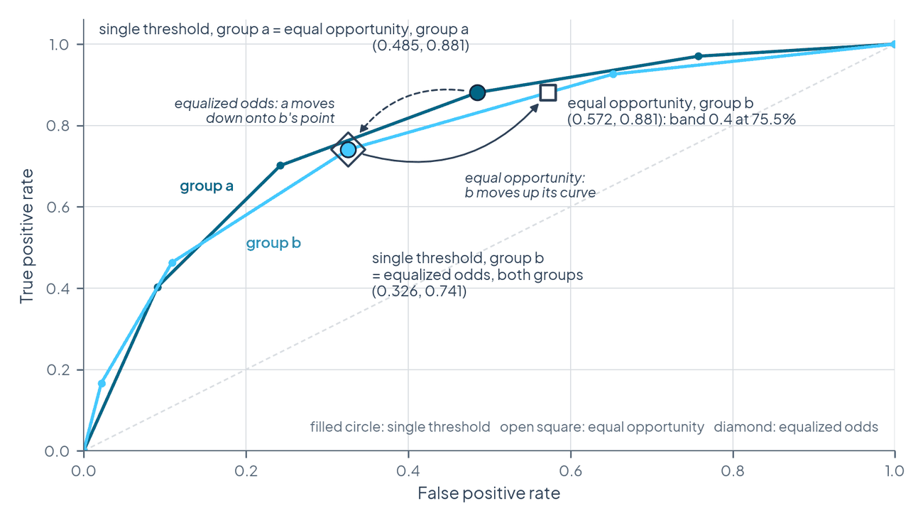
The fairness-utility frontier. Relaxing equal opportunity to |TPRa − TPRb| ≤ ε traces the frontier between the unconstrained rule and exact equal opportunity. In this example the frontier is a straight line, because the marginal approvals all come from the same band: each 2 percentage points of allowed TPR gap recover 2.7 units of profit (about 0.5 percent of the maximum).
| Allowed TPR gap ε | TPR a / b | Profit | Share of max |
|---|---|---|---|
| 0.00 | 0.881 / 0.881 | 536.1 | 96.6% |
| 0.04 | 0.881 / 0.841 | 541.5 | 97.6% |
| 0.08 | 0.881 / 0.801 | 546.9 | 98.5% |
| 0.12 | 0.881 / 0.761 | 552.3 | 99.5% |
| 0.14 | 0.881 / 0.741 | 555.0 | 100% |
Source: computed for this chapter.
Source: validant.ai.
The example also shows that the criteria can agree or disagree depending on the data. Here demographic parity and equal opportunity lead to almost the same decisions, because the gap in selection rates and the gap in true positive rates are both closed by approving more of group b's band-0.4 applicants. Equalized odds leads somewhere else entirely. An assessor should therefore compute every candidate criterion on the actual data before arguing about them in the abstract.
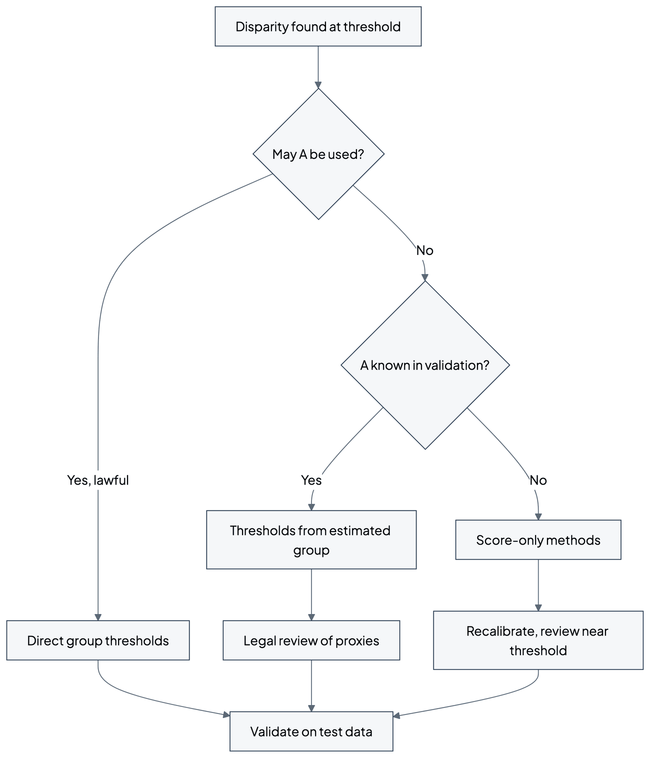
Deploying thresholds with and without the protected attribute
Direct group-specific thresholds
When the protected attribute is available at decision time and its use is lawful for this purpose, group-specific thresholds are applied directly. This gives the most flexible optimization and the exact targeting the theory describes. Common implementations require the attribute both when fitting and when predicting: the Fairlearn ThresholdOptimizer, which implements the Hardt et al. (2016) procedure, takes sensitive features as a required argument of its predict method and may return randomized predictions, controlled by a random seed (Fairlearn, n.d.-a).
Thresholds that depend on an estimate of group membership
Often the attribute may not be used at decision time, or is not even collected. In United States consumer credit, Regulation B generally prohibits a creditor from inquiring about the race, color, religion, national origin or sex of an applicant, with exceptions such as a voluntary self-test whose requirements the regulation sets out (12 CFR § 1002.5(b)). A second approach therefore trains, on validation data where group membership is known, a model that assigns thresholds from permissible features that correlate with group membership, and deploys only that model.
This approach has a precise theoretical counterpart. Menon and Williamson (2018) show that when the sensitive feature is not an input, the Bayes optimal classifier under a demographic parity penalty thresholds the class probability η(x) = P(Y = 1 | X = x) at a point that moves with the estimated probability of group membership, ηA(x) = P(A = 1 | X = x):
Here c is the cost parameter of the accuracy objective, c̄ that of the fairness measure and λ the weight given to fairness. The threshold rises for individuals who are confidently predicted to belong to the group whose selection rate is to be reduced, and falls for the others. For equal opportunity the correction is multiplicative instead of additive. When the features reveal group membership perfectly, the rule reduces to one constant threshold per group.
The approach is weaker and more fragile than direct thresholds. It achieves only part of the fairness effect, by an amount that depends on how well the features predict group membership, and it moves thresholds for individuals according to an estimate that may be wrong for them. It also does not escape the legal question it was built to avoid. Lipton, Chouldechova and McAuley (2018) show that when sensitive and nominally non-sensitive features are correlated, methods that use the sensitive attribute in training but produce a group-blind classifier indirectly implement treatment disparity, induce within-class discrimination when group membership is partly revealed by other features, and provide suboptimal trade-offs between accuracy and impact parity. A threshold model built on proxies is a direct instance of this pattern.
Rules that use the score alone
Without group information, a rule can only depend on the score. If acceptance is non-decreasing in the score, any such rule is a single (possibly randomized) threshold, which cannot reproduce group-specific thresholds. Score-only post-processing can still help in two ways: by recalibrating the score so that it means the same in every group (Chapter 56), and by routing uncertain cases near the threshold to human review or applying reject-option methods (Chapter 57). Learned representations that remove group information before scoring, such as adversarially trained ones (Chapter 53), act earlier in the pipeline and are not threshold methods.
| Option | Needs A at decision time | Fairness control | Main risk |
|---|---|---|---|
| Direct group thresholds | Yes | Exact, as optimized | Disparate treatment or direct discrimination |
| Thresholds from estimated group | No (needs A for training) | Partial | Treatment disparity by proxy; errors for individuals |
| Score-only threshold plus recalibration | No | Limited | Residual rate gaps remain |
| Human review near the threshold | No | Indirect | Reviewer bias; cost; inconsistency |
Source: compiled from Hardt et al. (2016), Menon and Williamson (2018), Lipton et al. (2018) and Fairlearn (n.d.-a).
Source: validant.ai.
The legal position
Group-specific thresholds are, on their face, a rule that treats people differently according to a protected characteristic. Whether this is permitted depends on the jurisdiction, the domain and the decision maker, and it is the first question to settle.
For public decision makers in the United States, Corbett-Davies et al. (2017) note that race-specific thresholds, under which a Black defendant may be released while an equally risky white defendant is detained, would likely trigger strict scrutiny under the Equal Protection Clause of the Fourteenth Amendment. In the European Union, the Fairlearn documentation observes that separate thresholds per group might be argued to constitute direct discrimination (Fairlearn, n.d.-b).
The EU AI Act addresses a related but distinct question. Regulation (EU) 2024/1689 as adopted allowed providers of high-risk AI systems, in Article 10(5), to process special categories of personal data exceptionally, where strictly necessary for bias detection and correction and subject to safeguards. The Digital Omnibus on AI, published in the Official Journal on 24 July 2026 and in force since 27 July 2026, extended this legal basis beyond providers of high-risk systems to deployers of high-risk systems and to providers and deployers of other AI systems and models, and retained the strict-necessity threshold (Lewis Silkin, 2026). In the consolidated text the permission sits in a new Article 4a, with conditions that include that the bias cannot be addressed with other data, including synthetic or anonymized data, that the data are pseudonymized and access-controlled, not transmitted to other parties, and deleted once the bias is corrected (AI Act Explorer, n.d.). Permission to process the data for detecting and correcting bias is not, by itself, permission to make individual decisions depend on the attribute.
Disparate impact doctrine is sometimes invoked in favor of group thresholds, on the reasoning that the law looks at effects. That is a misreading: in the United States, disparate impact is a ground of liability for facially neutral practices, not an authorization for group-conscious adjustments, and the employment provision quoted above expressly forbids one such adjustment. Where group-specific thresholds are lawful, their justification rests on documented evidence: the disparity under a common threshold, its connection to measurement problems or historical disadvantage, the narrowness of the adjustment and the alternatives considered.
Intersectionality
Threshold optimization over one attribute at a time can leave intersectional groups untreated. Buolamwini and Gebru (2018) evaluated three commercial gender classification systems on a data set balanced by gender and skin type and found that darker-skinned females were the most misclassified group, with error rates of up to 34.7 percent, against a maximum of 0.8 percent for lighter-skinned males; analyses by gender alone or by skin type alone hide the size of this gap. The same can happen with thresholds: equalizing true positive rates between women and men and between two ethnic groups does not equalize them for women of one ethnic group.
Applying threshold optimization intersectionally requires four things:
- A threshold for each relevant combination of attributes, optimized jointly, rather than separate adjustments for each attribute.
- Statistical methods for small groups, because intersectional cells are often small and their thresholds poorly estimated: pooling toward the parent group's threshold, Bayesian shrinkage, or a coarser grid of thresholds (Chapter 43).
- A prioritization rule for which intersectional disparities are addressed first, combining statistical evidence with the severity of harm.
- Monitoring of every intersection, not only of the main groups, since an adjustment for one group can move another.
As an illustration in facial analysis, an error pattern specific to young darker-skinned women would not be found by adjusting thresholds by gender or by skin type separately, and it needs its own operating point.
Implementation method
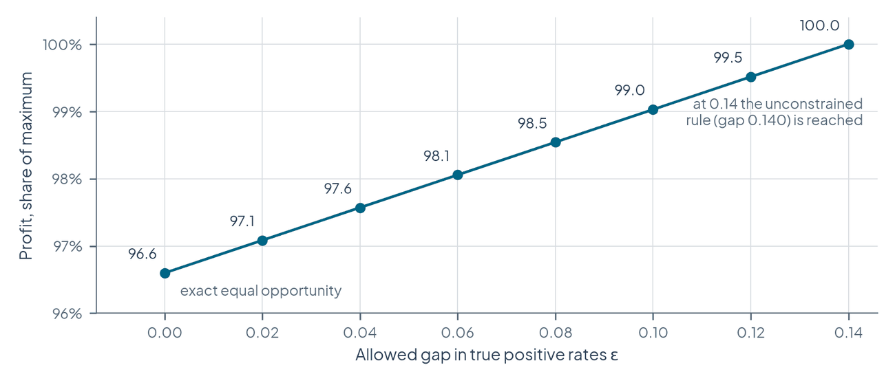
The following method organizes threshold optimization into four stages. It operates after training and is compatible with an existing deployment pipeline; it adds decision logic but requires no change upstream.
- Select the fairness criterion. Determine which criterion (demographic parity, equal opportunity, equalized odds) fits the context, using the selection reasoning of Chapter 22 and Chapter 44. Decide whether one criterion is optimized or several are balanced, and record the reasons, both normative and practical.
- Calculate thresholds. On validation data kept separate from both training and test data:
- for demographic parity, find thresholds that equalize selection rates;
- for equal opportunity, find thresholds that equalize true positive rates;
- for equalized odds, find thresholds that equalize true and false positive rates, which may require randomization between two thresholds in some groups.
3. Analyze trade-offs. Quantify how each candidate affects fairness metrics and performance, compute the fairness-utility frontier, select the final thresholds by an explicit prioritization of the competing objectives, and document the trade-off accepted.
4. Plan deployment. Establish whether the protected attribute may be used at decision time. If it may, implement direct thresholds; if not, consider the alternatives of the previous section and their legal review. Write implementation documentation for the production system.
A useful formalization of stage 2 for small problems is analytical: quantiles of each group's score distribution for demographic parity, and quantiles of each group's positive-class score distribution for equal opportunity. Larger or relaxed problems, intersectional grids and equalized odds are solved numerically, by linear programming on discretized scores or by search over the common operating point.
Domain modeling perspective
Threshold optimization touches five components of a machine learning system:
- Prediction interface: thresholds determine how continuous outputs become decisions that affect people.
- Fairness evaluation: every threshold choice changes the demographic parity, equal opportunity and equalized odds measures.
- Deployment pipeline: threshold logic must be integrated with production systems, possibly next to other interventions.
- Monitoring: thresholds may need adjustment as data distributions change.
- Compliance documentation: each threshold needs a recorded rationale for audit and transparency.
Because the intervention sits at the prediction interface, it is usually the easiest fairness intervention to integrate into an existing system.
Analogies
Three analogies, offered as analogies only, convey the idea.
- Qualifying times in a school athletics program. A school with one well-funded and one under-resourced training track might set different qualifying times for a state competition, so that students from both tracks have an equal chance of qualifying, recognizing that one standard applied to unequal preparation would carry the existing advantage forward. Group thresholds adjust a decision boundary in the same way to account for different score patterns across groups. The analogy is imperfect: in athletics the time measures the performance itself, whereas a model score is only an estimate of a future outcome.
- Precision and recall in search. A search engine must choose between showing more results (higher recall, lower precision) and fewer, more relevant ones (higher precision, lower recall). Threshold optimization makes the analogous choice between error types across groups, and no operating point optimizes every metric at once.
- Progressive taxation without income declarations by group. A tax schedule applies one set of brackets to everyone yet affects income groups differently. Threshold schemes based on permissible features act on groups without naming them at decision time. The analogy also carries the warning: the brackets work because income is the very quantity they act on, and a proxy-based threshold works only to the extent that the proxies encode group membership.
Practical challenges
Legal and ethical constraints
Many jurisdictions limit the use of protected attributes in decisions, even for mitigation. Practitioners should take legal advice for the specific context, design an implementation that approximates group thresholds without the attribute where that is the only lawful route, document the justification for any use of protected attributes, and turn to other interventions (Chapters 46 to 54) when threshold optimization meets a legal barrier it cannot clear.
Threshold stability
Thresholds tuned on validation data can perform differently in production. Distribution shift between groups, seasonal changes in applicant mix and changes in base rates all move the operating points that a fixed threshold produces. Lipton, Wang and Smola (2018) study label shift, in which the label distribution P(Y) changes while P(X | Y) stays fixed, and show how it can be detected and its new label distribution estimated from a black-box predictor's outputs; a change of this kind alters both the base rates and the meaning of a calibrated score, and so the thresholds that satisfy a criterion. Friedler et al. (2019) found in a comparative benchmark that fairness-preserving algorithms tend to be sensitive to fluctuations in data set composition, simulated by different training and test splits, which argues for estimating threshold variability before relying on a point estimate.
Stability is addressed by:
- estimating threshold variability by cross-validation or the bootstrap, and reporting confidence intervals around each threshold and around the resulting disparities (Chapter 41);
- monitoring the target rates per group in production and alerting when a disparity leaves its tolerance (Chapters 61 and 62);
- recalibrating thresholds periodically on recent labeled production data, with a documented procedure and a record of every change.
Resources
Threshold optimization needs validation data with reliable protected-attribute information, statistical expertise for estimation and evaluation, and monitoring infrastructure. These needs are lower than for pre-processing or in-processing, because neither the data pipeline nor the model is changed.
Evaluating a threshold intervention
Evaluation has two parts.
Fairness. Measure the target metrics (for example, the demographic parity difference or the equal opportunity difference) before and after adjustment, with confidence intervals to establish that the improvement is not sampling noise. Evaluate intersectional groups, not only the main groups. Verify the improvement on held-out test data, not only on the validation data used to fit the thresholds, since thresholds fitted to a sample overstate the parity they achieve.
Performance. Quantify the change in accuracy, precision, recall, F1 or the application's own utility, overall and for each group separately, so that no group suffers an unacceptable loss. Compute the efficiency of the intervention, the fairness gained per unit of performance lost, and compare it with the efficiency of pre-processing and in-processing alternatives. These measures belong in the organization's general fairness assessment (Chapter 36).
Illustrative scenario: a loan application system
The following scenario is illustrative; its numbers describe the scenario and are not empirical findings.
Context. A financial institution uses a model that outputs a predicted probability of default between 0 and 1 and rejects an application when the score exceeds a threshold, originally 0.5 for everyone. A fairness analysis finds that the model's true positive rate, here the share of non-defaulting applicants who are approved, is 85 percent for one racial group and 70 percent for another, despite similar actual default rates. Risk management wants accurate default prediction, compliance officers monitor fair lending obligations under the Equal Credit Opportunity Act, and business leaders balance growth against risk. Retraining would take months of development and validation, whereas new thresholds could be introduced quickly.
Analysis. Because the concern is qualified applicants being rejected, equal opportunity is the appropriate criterion. Group ROC curves show that the common threshold produces different rates because the score distributions differ, plausibly reflecting historical patterns in the lending data. Computing the frontier shows that equal true positive rates require a stricter rejection cutoff for the advantaged group (reject above a default probability of 0.45) and a more lenient one for the disadvantaged group (reject above 0.65), at a projected profit reduction of about 3 percent. Legal counsel advises that using race explicitly, even for mitigation, could breach regulatory guidance, so direct thresholds are ruled out. An intersectional analysis finds the disparity strongest for younger applicants in the disadvantaged group, with a true positive rate of 60 percent.
Implementation. The team computes the equal opportunity thresholds on validation data with protected attributes; they bring both groups' true positive rates to about 80 percent, between the original 85 and 70 percent, and a statistical test confirms the reduction. Because race may not be used, the team trains a small threshold-assignment model on legally permissible features that correlate with group membership; in validation it recovers about 90 percent of the fairness gain of direct thresholds. Age, a permissible feature in this setting, lets the model partly address the intersectional disparity. The team monitors true positive rates for all groups and intersections, with alerts when a disparity exceeds a set limit, and holds quarterly reviews of fairness and business impact. Every threshold change is documented as an audit trail.
Outcomes. In production the true positive rate gap falls from 15 percentage points to about 3, a reduction of 80 percent. The profit reduction is 1.8 percent rather than the projected 3 percent, because additional lending to qualified applicants of the disadvantaged group offsets part of the loss. The intersectional disparity improves but is not resolved.
Lessons. The proxy scheme needed careful legal review for treatment disparity by proxy, which Lipton et al. (2018) show is what such schemes implement. The thresholds had to be adjusted after two months because of seasonal changes in the applicant mix. Business stakeholders understood the trade-off only when it was stated in currency rather than in rates. Threshold optimization gave a quick improvement without retraining, but resolving the intersectional disparity required longer-term data collection and model improvement.
A Threshold Optimization Method
The material of this chapter can be organized into a reusable method with three components.
- Threshold calculation framework. Step-by-step procedures for each criterion: analytical quantile solutions for demographic parity and equal opportunity with continuous scores, and numerical optimization (linear programming on discretized scores, search over the common operating point) for equalized odds, relaxed constraints and intersectional grids.
- Trade-off analysis. Frontier computation, standard visualizations (group ROC curves with operating points, utility against tolerance) and a decision record of the chosen point and its rationale.
- Implementation patterns by constraint. Direct group thresholds where the attribute may be used, thresholds from estimated group membership with legal review where it may not, and score-only measures with human review where no group information is available, with criteria for choosing among them.
The method interfaces with the other post-processing methods. Recalibration (Chapter 56) ensures that scores mean the same in every group before thresholds are set, and should normally precede threshold optimization. Prediction transformation (Chapter 57) generalizes thresholds to other mappings, including reject-option classification. Shared notation, documented assumptions and common evaluation metrics make the three combinable.
Competing interpretations and limitations
Equal treatment against equal impact. A single threshold treats equal scores equally; group thresholds equalize rates. Each realizes a different idea of fairness, and Corbett-Davies et al. (2017) present the single threshold as satisfying one important understanding of equality, holding everyone to the same standard. The choice is normative and cannot be settled by the optimization.
The score's validity. Threshold optimization takes the score and the labels as given. If the labels are biased, for example because repayment is observed only for previously approved applicants (Chapter 12, selective labels), equalizing rates measured against those labels may not equalize anything that matters. Chapter 15 discusses label bias for separation in detail.
Leveling down and randomization. Exact equalized odds can require worsening outcomes for the better-served group and deciding by chance. Both are reasons to prefer equal opportunity or a relaxed criterion in many settings, and both deserve explicit justification when accepted.
Impossibility. Threshold adjustment cannot escape the impossibility results of Chapter 19. Kleinberg, Mullainathan and Raghavan (2017) prove that, except in highly constrained special cases (equal base rates or perfect prediction), no method satisfies calibration within groups and balance for both the positive and the negative class at once. Group thresholds that equalize error rates will in general make the positive predictive value differ between groups, as the worked example shows (PPV of 0.787 against 0.644 under equal opportunity).
Static optimization in a dynamic world. Thresholds are fitted to a snapshot. Changing them changes who receives credit or a job, which changes future data and future base rates. Chapter 27 discusses such feedback loops.
Common questions
Does using different thresholds for different groups violate the principle of treating everyone equally?
It departs from one principle in favor of another. A single threshold is procedurally equal, since everyone faces the same rule, but it can produce unequal outcomes when score distributions or score quality differ for reasons linked to historical disadvantage or measurement problems. Group thresholds trade procedural sameness for equal error rates or equal selection rates. Ethically, the case for them rests on documented evidence: the disparity under a single threshold, its link to measurement or historical discrimination, the narrow targeting of the adjustment and the alternatives considered. Legally, the position differs by domain and jurisdiction. In United States employment, different cutoff scores by race, color, religion, sex or national origin are expressly prohibited (42 U.S.C. § 2000e-2(l)); disparate impact law does not authorize such adjustments; in the European Union the practice may be argued to be direct discrimination. Legal advice for the specific case is indispensable.
How can threshold optimization be implemented when the protected attribute is unavailable at decision time or may not be used?
Three routes exist. A threshold-assignment model can be trained on validation data with the attribute and deployed on permissible features that correlate with it; Menon and Williamson (2018) characterize the optimal rule of this kind as an instance-dependent threshold that moves with the estimated probability of group membership. Score-only measures, such as per-group recalibration fitted offline and human review near the threshold, require no group information at decision time. Representations that remove group information can be learned earlier in the pipeline (Chapter 53). Each route achieves less than direct thresholds, by an amount that depends on the data and must be measured on validation data with the attribute; no general percentage can be assumed. The first route also needs legal review, because it implements treatment disparity by proxy (Lipton et al., 2018). The methodology should be documented in full.
Is threshold optimization a good first intervention?
For an organization new to fairness interventions it often is, because it is simple, quick and does not disrupt the model. It provides an immediate improvement while more fundamental interventions, such as better data or a retrained model, are developed. It should not be mistaken for a final fix when the underlying score is poor for some groups.
Should thresholds be set before or after recalibration?
After. If the score means different things in different groups, thresholds on it compound the confusion. Recalibrating first (Chapter 56) gives thresholds a common interpretation, and threshold optimization then addresses the error-rate and selection-rate criteria that calibration cannot.
Conclusions
Threshold optimization is the most direct way to make a fixed score satisfy a group fairness criterion. The theory is clear: under a parity constraint, the utility-maximizing rule is a group-specific threshold rule, equal opportunity needs only deterministic thresholds when scores are continuous, and equalized odds needs randomization and moves the better-served group onto the lower ROC curve. The practical questions are what determines whether the method is appropriate: whether the attribute may be used at decision time, whether randomized or group-dependent decisions are acceptable in the domain, how much utility the chosen point costs, and whether the thresholds remain valid as the population changes.
Methodologically, the method's value lies in transparency. Computing the frontier, reporting per-group rates and utility with their uncertainty, and documenting the chosen point and its legal basis turn an implicit choice (one threshold for everyone) into an explicit, auditable decision. Threshold optimization should normally follow recalibration, be validated on held-out data and in production, and be combined with longer-term improvement of data and models where the score itself is the problem.
Open questions
- How should the acceptability of randomized decisions be judged in domains where individuals have a right to a reasoned decision?
- Under which conditions, if any, may thresholds that depend on an estimate of group membership be lawful where direct thresholds are not?
- How should intersectional thresholds be estimated and governed when many cells are small?
- What is the right cadence and statistical procedure for re-estimating thresholds under distribution shift without causing instability in decisions?
- How do threshold interventions interact over time with the data they generate, and when do they improve or worsen future scores for the disadvantaged group?
References
- AI Act Explorer. (n.d.). Article 4a: Processing of special categories of personal data for bias detection and correction. Retrieved November 5, 2026, from https://artificialintelligenceact.eu/article/4a/
- Buolamwini, J., & Gebru, T. (2018). Gender shades: Intersectional accuracy disparities in commercial gender classification. In Proceedings of the 1st Conference on Fairness, Accountability and Transparency (Proceedings of Machine Learning Research, Vol. 81, pp. 77 - 91). https://proceedings.mlr.press/v81/buolamwini18a.html
- Corbett-Davies, S., Pierson, E., Feller, A., Goel, S., & Huq, A. (2017). Algorithmic decision making and the cost of fairness. In Proceedings of the 23rd ACM SIGKDD International Conference on Knowledge Discovery and Data Mining (pp. 797 - 806). ACM. https://doi.org/10.1145/3097983.3098095
- Equal Credit Opportunity Act, 15 U.S.C. § 1691. https://www.law.cornell.edu/uscode/text/15/1691
- Equal Credit Opportunity Act (Regulation B), 12 C.F.R. § 1002.5. https://www.law.cornell.edu/cfr/text/12/1002.5
- Fairlearn. (n.d.-a). fairlearn.postprocessing.ThresholdOptimizer. Retrieved November 5, 2026, from https://fairlearn.org/main/api_reference/generated/fairlearn.postprocessing.ThresholdOptimizer.html
- Fairlearn. (n.d.-b). Postprocessing. Fairlearn user guide. Retrieved November 5, 2026, from https://fairlearn.org/main/user_guide/mitigation/postprocessing.html
- Friedler, S. A., Scheidegger, C., Venkatasubramanian, S., Choudhary, S., Hamilton, E. P., & Roth, D. (2019). A comparative study of fairness-enhancing interventions in machine learning. In Proceedings of the Conference on Fairness, Accountability, and Transparency (pp. 329 - 338). ACM. https://doi.org/10.1145/3287560.3287589
- Hardt, M., Price, E., & Srebro, N. (2016). Equality of opportunity in supervised learning. In Advances in Neural Information Processing Systems 29. https://arxiv.org/abs/1610.02413
- Kleinberg, J., Mullainathan, S., & Raghavan, M. (2017). Inherent trade-offs in the fair determination of risk scores. In 8th Innovations in Theoretical Computer Science Conference (ITCS 2017) (Leibniz International Proceedings in Informatics, Vol. 67, pp. 43:1 - 43:23). https://doi.org/10.4230/LIPIcs.ITCS.2017.43
- Lewis Silkin. (2026, July 27). The Digital Omnibus on AI enters into force today. https://www.lewissilkin.com/insights/2026/07/27/the-digital-omnibus-on-ai-enters-into-force-today-102nedo
- Lipton, Z. C., Chouldechova, A., & McAuley, J. (2018). Does mitigating ML's impact disparity require treatment disparity? In Advances in Neural Information Processing Systems 31. https://arxiv.org/abs/1711.07076
- Lipton, Z. C., Wang, Y.-X., & Smola, A. (2018). Detecting and correcting for label shift with black box predictors. In Proceedings of the 35th International Conference on Machine Learning (Proceedings of Machine Learning Research, Vol. 80, pp. 3122 - 3130). https://proceedings.mlr.press/v80/lipton18a.html
- Menon, A. K., & Williamson, R. C. (2018). The cost of fairness in binary classification. In Proceedings of the 1st Conference on Fairness, Accountability and Transparency (Proceedings of Machine Learning Research, Vol. 81, pp. 107 - 118). https://proceedings.mlr.press/v81/menon18a.html
- Regulation (EU) 2024/1689 of the European Parliament and of the Council of 13 June 2024 laying down harmonised rules on artificial intelligence (Artificial Intelligence Act). Official Journal of the European Union, L, 2024/1689. https://eur-lex.europa.eu/eli/reg/2024/1689/oj
- Title VII of the Civil Rights Act of 1964, 42 U.S.C. § 2000e-2(l) (prohibition of discriminatory use of test scores). https://www.law.cornell.edu/uscode/text/42/2000e-2