Multi-Objective Optimization

Overview

Every fairness intervention discussed so far in Part V touches more than one goal at once. A constraint (Chapter 51) caps a disparity while the learner minimizes error; a penalty (Chapter 52) adds a weighted disparity term to the loss; an adversary (Chapter 53) trades task accuracy against how much the protected attribute can be recovered. Each method contains a dial, a constraint bound, a penalty weight λ or an adversary weight, and each setting of the dial yields a different compromise. Treating that dial as an ordinary hyperparameter hides a decision that is not technical at all: how much predictive performance an organization accepts to give up for how much reduction in disparity, and which disparity it cares about most.

Multi-objective optimization makes the decision explicit. Instead of folding fairness into a single objective in advance, it models performance and each fairness criterion as separate objectives, computes the set of models that are not beaten on every objective at once, and presents that set for an informed choice. The central concept is Pareto optimality: a model is Pareto optimal if no other available model is at least as good on every objective and strictly better on one. The set of Pareto optimal models, viewed in the space of objective values, is the Pareto front or frontier. Constraints, penalties and adversaries then appear as different ways of reaching points on the same frontier.

This matters most in high-stakes settings, such as credit, hiring and healthcare, where both fairness and performance carry real consequences and several stakeholders hold different priorities. It also matters for assurance: a reviewer who sees only the chosen model cannot tell whether a better compromise existed, while a reviewer who sees the frontier and the documented reasons for the choice can. The chapter builds on the fairness criteria of Chapters 14 to 16, on the impossibility and trade-off results of Chapters 19 and 20, and on Chapters 51 to 53. Chapter 55 takes up a related option, moving the trade-off from training into the decision thresholds.

Learning objectives:

• Explain why fairness-aware learning is a multi-objective problem and where the tension between fairness and performance comes from.
• Define Pareto dominance, Pareto optimality, weak Pareto optimality, the Pareto front and the utopia point, and test a set of candidate models for dominance.
• Compare linear scalarization, the ε-constraint method, Chebyshev scalarization, boundary-intersection methods, randomized mixtures and evolutionary algorithms for generating a fairness-performance frontier.
• Show by calculation why a weighted sum cannot reach compromise models on non-convex parts of a frontier.
• Organize a priori, a posteriori and interactive preference articulation and document the value judgments behind an operating point.
• Handle intersectional and many-objective formulations and evaluate a frontier with dominance checks and the hypervolume indicator.

Key questions

• How can the tension between fairness criteria and conventional performance metrics be navigated systematically during model development?
• Which methods support principled trade-off decisions, rather than ad hoc compromises, when several objectives conflict?
• Which compromises can a given method find, and which can it never find?
• Who decides where on the frontier a model should operate, at what point in the process, and how is that decision recorded?
• How does the problem change when fairness must hold for intersectional subgroups and the number of objectives grows?
• How can the quality of a computed frontier be assessed?

Definitions and terminology

Objective. A quantity to be minimized or maximized, for example the error rate, one minus the area under the ROC curve (AUC), the demographic parity difference, or the gap in true positive rates (TPR_a minus TPR_b). In this chapter every objective is written so that smaller is better.

Multi-objective optimization problem. The task of minimizing a vector of objectives F(θ) = (f₁(θ), ..., f_k(θ)) over model parameters θ, when no single θ minimizes all of them at once.

Pareto dominance. Model θ′ dominates model θ if θ′ is no worse on every objective and strictly better on at least one.

Pareto optimal (non-dominated) model. A model that no other feasible model dominates. A model is weakly Pareto optimal if no other model is strictly better on every objective simultaneously; every Pareto optimal model is weakly Pareto optimal, but not the reverse (Wei & Niethammer, 2022).

Pareto set and Pareto front. The Pareto set is the set of Pareto optimal solutions in decision (parameter) space; its image in objective space is the Pareto front (Guerreiro et al., 2022). In fairness work the front is often called the fairness-accuracy frontier.

Utopia point. The vector of the best values each objective can reach on its own. It is usually unattainable, since the objectives conflict, and serves as a reference for several methods.

Scalarization. Turning a vector of objectives into a single number to be optimized, for example a weighted sum. Each choice of the scalarization's parameters yields one candidate point on the front.

Preference articulation. The way the decision maker's priorities enter the process: before the search (a priori), after the front has been computed (a posteriori), or repeatedly during the search (interactive) (Emmerich & Deutz, 2018).

Operating point. The model, and so the point on the front, that is finally selected for deployment.

Hypervolume indicator. The size of the region of objective space that a set of points dominates, bounded by a reference point; a single-number measure of the quality of a front approximation (Guerreiro et al., 2022).

Why fairness is a multi-objective problem

Where the tension comes from

Fairness criteria and performance metrics conflict for structural reasons, not only because of imperfect implementations. Corbett-Davies et al. (2017) cast pretrial release decisions as constrained optimization: maximize public safety subject to a formal fairness constraint. They show that for several common fairness definitions the optimal constrained rule detains defendants above race-specific risk thresholds, whereas the optimal unconstrained rule applies one uniform threshold to everyone. Because the two optima differ, satisfying the fairness definition costs some of the primary objective, and on data from Broward County, Florida, they find that this cost can be large in practice.

The mechanism is general. When base rates differ between groups (p_a ≠ p_b), a criterion such as demographic parity (Chapter 14) can only be met by treating otherwise similar scores differently by group or by withholding predictive information that is correlated with the protected attribute. In a loan approval model, enforcing demographic parity may require downweighting features that genuinely predict default but are also correlated with group membership, which reduces the model's ability to predict default risk. Fairness criteria can also conflict with one another: the impossibility results of Chapter 19 show that calibration within groups and equal error rates cannot hold together when base rates differ, except in degenerate cases.

These conflicts are the reason multi-objective formulations are needed. Unlike a problem with one well-defined goal, fairness-aware learning involves competing goals that cannot all be pushed to their individual optima at once. The tension must be modeled explicitly rather than absorbed silently into a tuned hyperparameter.

A large trade-off is a diagnostic signal

A frontier is also evidence about the data. Agarwal, Dudík and Wu (2019), who use their reduction algorithms to uncover fairness-accuracy frontiers, advise that any substantial trade-off along the frontier be analyzed: it may point to data problems that call for non-algorithmic remedies, such as collecting additional, less biased data or adding new features. They add that the societal context of the application must be considered and that in some contexts the best intervention may be to avoid a technological intervention altogether. A steep frontier is therefore a prompt to revisit data collection (Chapter 25) and the choice of label, not only a menu of compromises.

Analogies

Three analogies from the source material help fix the ideas; they are analogies, not technical claims about those fields.

• Fuel economy and acceleration. A car cannot maximize fuel economy and acceleration at the same time, so manufacturers offer models along a spectrum from economy cars to sports cars. In the same way a model cannot always maximize performance and certain fairness criteria together when base rates differ, and a team can produce a range of models along the frontier and select the one the application requires.
• Risk and return in a portfolio. A portfolio is efficient if no other portfolio offers a higher return at the same risk or a lower risk at the same return, and advisers present clients with this efficient frontier to choose according to their risk tolerance. A model is Pareto optimal in the same sense, and the frontier of models can be presented to stakeholders who choose according to their priorities and fairness requirements.
• Planning a diet. Some people fix nutritional requirements first and then consider taste (a priori), some sample many options and then pick the best balance (a posteriori), and some adjust their diet over time based on both nutritional feedback and taste (interactive). Organizations articulate fairness and performance preferences in the same three ways.

The formal framework

The multi-objective problem

Write each objective so that smaller is better. A typical fairness formulation has one performance objective and one or more fairness objectives:

For example f₁ may be the error rate, f₂ the demographic parity difference |P(Ŷ = 1 | A = a) − P(Ŷ = 1 | A = b)| and f₃ the equal opportunity difference |TPR_a − TPR_b|. The problem has no single solution because improving one component usually worsens another.

Dominance and Pareto optimality

Model θ′ dominates model θ when

A model θ* is Pareto optimal if no feasible θ′ dominates it. It is weakly Pareto optimal if there is no θ′ with f_i(θ′) < f_i(θ*) for every i. The Pareto front is the set of objective vectors F(θ*) of all Pareto optimal models (Wei & Niethammer, 2022; Guerreiro et al., 2022). The utopia point collects the individual minima:

Every point on the front embodies a trade-off: accuracy cannot be improved without increasing unfairness, and unfairness cannot be reduced without losing accuracy. In a credit scoring application, the front may run from the most accurate model with no fairness intervention to a model with perfect demographic parity and lower predictive performance, with a continuum of compromises in between. Dominated models, by contrast, are never defensible choices: some other model is better on at least one objective and no worse on any.

Group risks as objectives: minimax Pareto fairness

The objectives need not be one performance metric plus disparity metrics. Martinez, Bertran and Sapiro (2020) formulate group fairness as a multi-objective problem in which each protected group's risk is a separate objective. Pareto optimality then expresses "no unnecessary harm": on the front, any increase in one group's risk is matched by a decrease in another's. Among the Pareto efficient classifiers they select the one with the smallest worst-group risk, which they call minimax Pareto fairness. This rule does not force equal risks if equalizing would only make the better-off group worse without helping the disadvantaged group; if policy nevertheless demands a zero gap, a deliberately harmful post-hoc correction can be added, a choice they leave to the policymaker. Their method does not require the protected attribute at test time, and they evaluate it on income prediction (Adult), intensive care mortality from clinical notes (MIMIC-III), skin lesion classification (HAM10000) and credit risk (German Credit).

The formulation also clarifies when simple weighting is enough. Martinez et al. (2020) prove that when the hypothesis class is convex and the group risks are convex, the Pareto front is convex and every efficient classifier can be recovered by minimizing a linear weighting of the group risks. The next section shows what goes wrong when those conditions fail.

Generating the frontier

Linear scalarization

The most common method combines the objectives in a weighted sum. For a performance loss and a fairness loss with λ ∈ [0, 1]:

and, for k objectives with positive weights w_i,

Training one model for each of a grid of weights traces a set of candidate points. The bounded form is equivalent to the unbounded penalty form L_perf + λ′ L_fair of Chapter 52, with λ′ = λ/(1 − λ) for λ < 1, since multiplying an objective by the positive constant 1/(1 − λ) does not change its minimizer. Fairness regularization (Chapter 52) is this method with a single fixed weight: a penalty of the form error(θ) + λ × unfairness(θ) is a linear scalarization, and Wei and Niethammer (2022) note that many train-time fairness methods take this form. Multi-objective practice differs mainly in intent: it sweeps the weights deliberately to map the range of trade-offs rather than committing to one setting in advance.

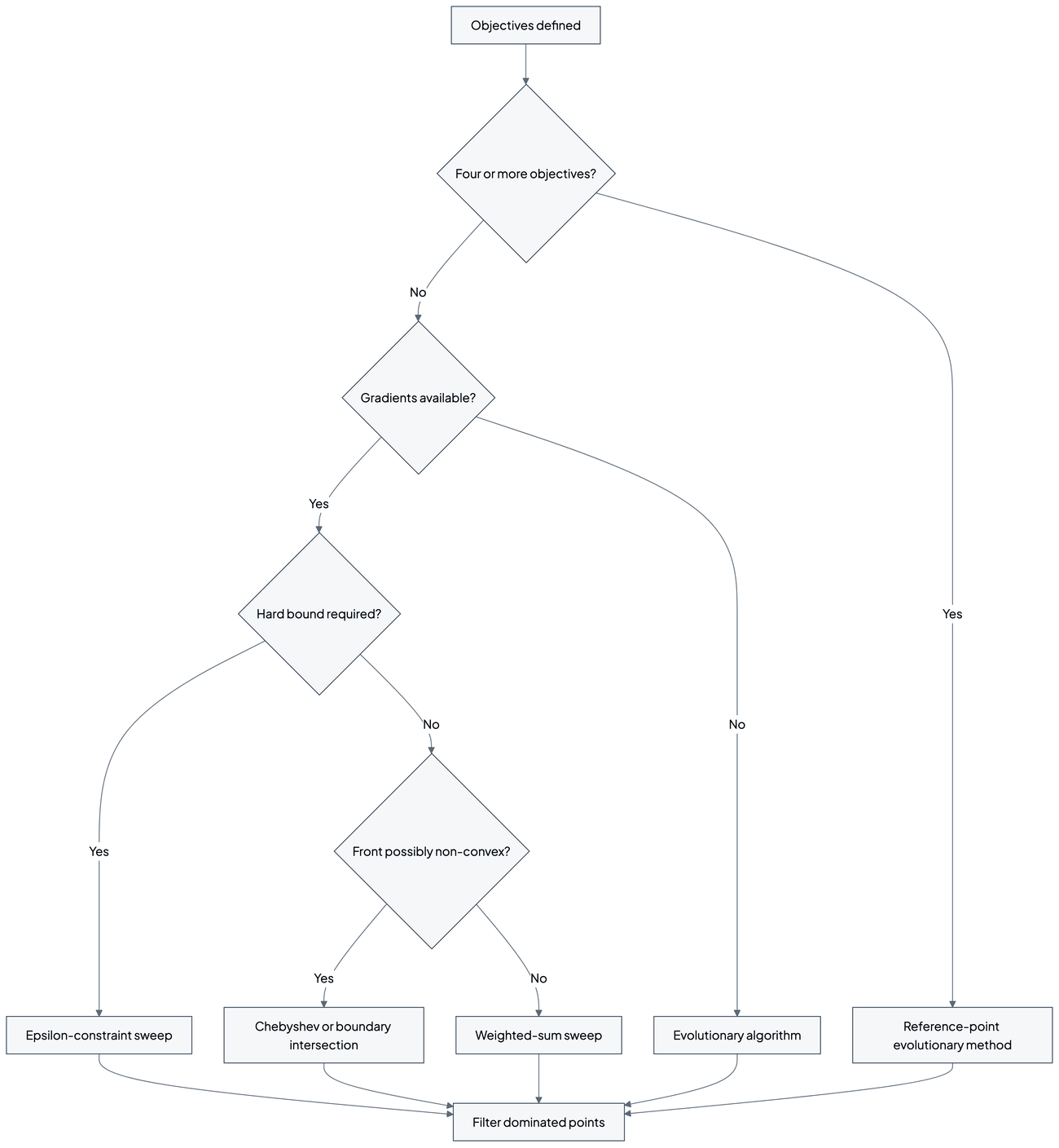
Linear scalarization has two limitations. First, it can only recover points on the convex hull of the Pareto front; points in non-convex regions are Pareto optimal but are never the minimizer of any weighted sum (Das & Dennis, 1997; Wei & Niethammer, 2022). Using more weights, with a finer step, does not cure this. Second, an even spread of weights does not produce an even spread of solutions along the front, so some regions are sampled densely and others hardly at all (Kim & de Weck, 2005). The objectives should also be put on comparable scales before weighting, since the meaning of a weight depends on the units of each objective. On the positive side, a minimizer of a weighted sum is always at least weakly Pareto optimal (Wei & Niethammer, 2022), and under the convexity conditions of Martinez et al. (2020) the weighted sum reaches the whole front.

The ε-constraint method

The ε-constraint method keeps one objective as the target and turns the others into constraints (Emmerich & Deutz, 2018):

Varying the bounds ε_i yields different points on the front, including points in non-convex regions, although weakly dominated solutions can also appear and should be filtered out. The method fits applications where a minimum performance level or a maximum disparity must be maintained, because the bound has a direct meaning. The constraint-based learners of Chapter 51 are ε-constraint solvers. Zafar et al. (2017, 2019) bound the covariance between the protected attribute and the signed distance to the decision boundary by a threshold c; in their synthetic experiments, a smaller threshold led to a fairer solution at a larger cost in accuracy (Zafar et al., 2017). They also use the reverse formulation, maximizing fairness subject to fine-grained accuracy constraints (Zafar et al., 2017), which is the same method with the roles of the objectives exchanged. The reductions approach of Agarwal et al. (2018) likewise returns the classifier with the lowest empirical error subject to the desired fairness constraints, and its slack parameter serves as a tunable knob for navigating the trade-off (Agarwal, Dudík & Wu, 2019).

Chebyshev scalarization

The Chebyshev (Tchebycheff) scheme minimizes the largest weighted distance from the utopia point (Wei & Niethammer, 2022):

Its solutions are at least weakly Pareto optimal, and every Pareto optimal solution can be obtained for some choice of weights, so unlike the weighted sum it can reach non-convex parts of the front. Wei and Niethammer (2022) apply it to estimate the fairness-accuracy front of a neural network classifier and argue that it is no more computationally burdensome than linear scalarization while being theoretically superior when the front is non-convex, as it may well be. In practice z* is approximated by the best value each objective reaches in single-objective runs.

Boundary intersection and adaptive weighting

Two families address the uneven spread of weighted sums. Normal-boundary intersection (Das & Dennis, 1998) sends search rays from evenly spaced reference points on the line (with two objectives) or hyperplane (with more) through the single-objective optima and finds where each ray meets the attainable set (Emmerich & Deutz, 2018). The evenly spaced starting points give an evenly spread set of solutions, but the points returned should still be checked for dominance, since on strongly curved boundaries an intersection point need not be Pareto optimal. The adaptive weighted-sum method (Kim & de Weck, 2005) starts with a coarse weighted sum and then refines the search in regions of the front where solutions are sparse, which lets it find solutions in non-convex regions while discarding dominated ones.

Randomized mixtures

A model owner can also combine two trained models by randomization: for each case, use model 1 with probability q and model 2 otherwise. Both the expected error and each group's selection rate are then the corresponding weighted averages, so the mixture lies on the straight line between the two models in objective space whenever the disparity has the same sign for both. Agarwal et al. (2018) build on this: their reductions yield a randomized classifier, and Agarwal, Dudík and Wu (2019) use randomized predictors explicitly to achieve better fairness-accuracy trade-offs. Randomization fills in the convex hull of the attainable points, which can dominate a deterministic model in a non-convex dent of the front, as the worked example below shows. Its cost is that two identical applicants can receive different decisions by chance, which raises questions of individual fairness (Chapter 17), consistency and explainability that must be addressed before deployment.

Evolutionary multi-objective algorithms

Evolutionary algorithms search for many non-dominated solutions concurrently in a single run (Zitzler & Thiele, 1999). The strength Pareto evolutionary algorithm (SPEA) keeps an external archive of non-dominated solutions and assigns fitness by dominance (Zitzler & Thiele, 1999); NSGA-II (Deb et al., 2002) ranks a population by non-dominated sorting and preserves diversity with a crowding distance (Emmerich & Deutz, 2018). For four or more objectives, NSGA-III (Deb & Jain, 2014) emphasizes non-dominated members close to a set of supplied reference points and was tested on problems with three to 15 objectives. These methods do not need gradients, which suits non-differentiable fairness metrics and model classes such as decision trees. Valdivia, Sánchez-Monedero and Casillas (2021) use a multi-objective framework to explore the Pareto front between accuracy and fairness for logistic regression and decision tree classifiers, with the stated aim of helping stakeholders assess how far they can go in being both fair and accurate.

Method	Parameter varied	Reaches non-convex regions	Typical fairness use
Linear scalarization	Weights wi or λ	No (convex hull only)	Penalized losses (Chapter 52)
ε-constraint	Bounds εi	Yes (filter weak points)	Constrained learning (Chapter 51)
Chebyshev scalarization	Weights λi, utopia z*	Yes	Neural network fronts
Boundary intersection, adaptive weights	Reference points, refined weights	Yes (with Pareto filter)	Even coverage of a front
Randomized mixture	Mixing probability q	Fills the convex hull	Reductions approach
Evolutionary algorithms	Population, reference points	Yes (approximate)	Many objectives, non-differentiable metrics

Source: Das and Dennis (1997, 1998); Kim and de Weck (2005); Emmerich and Deutz (2018); Wei and Niethammer (2022); Agarwal et al. (2018); Deb and Jain (2014).

Source: validant.ai.

Worked example: seven candidate credit models

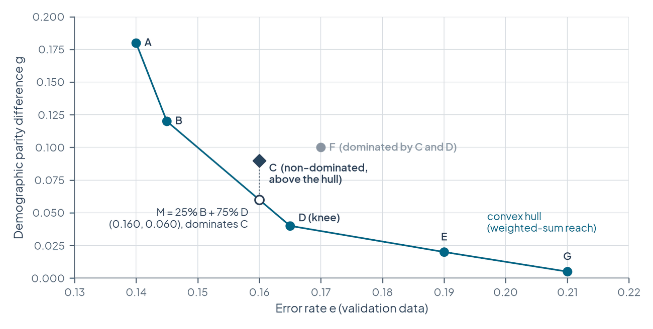
A lender trains seven candidate default-prediction models with different fairness settings and measures two objectives on validation data: the error rate e and the absolute demographic parity difference g between two groups. The figures are illustrative, chosen to show the mechanics; all derived numbers below were computed in Python.

Model	Error rate e	Accuracy	DP difference g	Status
A	0.140	86.0 percent	0.180	Non-dominated
B	0.145	85.5 percent	0.120	Non-dominated
C	0.160	84.0 percent	0.090	Non-dominated
D	0.165	83.5 percent	0.040	Non-dominated
E	0.190	81.0 percent	0.020	Non-dominated
F	0.170	83.0 percent	0.100	Dominated by C and D
G	0.210	79.0 percent	0.005	Non-dominated

Dominance. F is dominated twice: C has a lower error (0.160 against 0.170) and a lower gap (0.090 against 0.100), and D is also better on both. No other model dominates A, B, C, D, E or G, so these six form the empirical front. F should never be chosen, whatever the stakeholders' priorities.

Marginal cost of fairness. Moving along the front from A to G, the extra error per point of disparity removed is 0.083 (A to B: 0.5 points of error for 6 points of gap), 0.500 (B to C: 1.5 for 3), 0.100 (C to D: 0.5 for 5), 1.250 (D to E: 2.5 for 2) and 1.333 (E to G: 2.0 for 1.5). Two features stand out. The cost jumps after D, so D sits at the knee where further fairness becomes expensive. And the sequence is not increasing: the step into C is dearer than the step out of it. That is the signature of a non-convex dent in the front at C.

What a weighted sum finds. Minimizing (1 − λ)e + λg, the selected model switches where two models tie, that is, where λ/(1 − λ) equals the marginal cost between neighbors on the convex hull. The switches fall at λ = 0.0769 (A to B), λ = 0.2 (B to D), λ = 0.5556 (D to E) and λ = 0.5714 (E to G). Model C is never selected for any λ. On an evenly spaced grid of 101 values of λ from 0 to 1, A is chosen 8 times, B 13 times, D 35 times, E only 2 times, G 43 times and C never (at λ = 0.2 B and D tie exactly; the count gives that grid point to B). Both limitations of linear scalarization appear at once: a Pareto optimal model is unreachable, and the even grid of weights concentrates on a few models.

The geometry explains it. On the straight line from B to D, the point with C's error rate (0.160, three quarters of the way from B) has a gap of 0.060. C's gap of 0.090 lies above that line, so C is not on the convex hull of the front.

What the ε-constraint method finds. Minimizing error subject to g ≤ ε selects B for ε = 0.15, C for ε = 0.10, D for ε = 0.05, E for ε = 0.03 and G for ε = 0.01. The bound reaches C, and each bound has a direct meaning that stakeholders can discuss.

What Chebyshev scalarization finds. With the utopia point approximated by the best observed values, z* = (0.140, 0.005), and weights w on error and 1 − w on the gap, a grid of w from 0.01 to 0.99 selects G for w from 0.01 to 0.17, E from 0.18 to 0.41, D from 0.42 to 0.77, C from 0.78 to 0.85, B from 0.86 to 0.97 and A at 0.98 and 0.99. At w = 0.80, for example, C scores max(0.8 × 0.020, 0.2 × 0.085) = 0.017, against 0.020 for D and 0.023 for B. Every non-dominated model is reachable.

What randomization adds. A mixture that uses B for 25 percent of cases and D for 75 percent has an expected error of 0.25 × 0.145 + 0.75 × 0.165 = 0.160 and, if both models favor the same group, a gap of 0.25 × 0.120 + 0.75 × 0.040 = 0.060. It matches C's error and has a smaller gap, so it dominates C. Whether the lender should prefer a randomized policy over C is not settled by this arithmetic; it depends on whether chance-based treatment of applicants is acceptable.

Hypervolume. With the reference point r = (0.25, 0.20), the six non-dominated models dominate an area of 0.01725 in (error × gap) units. Removing a single model reduces the area by its contribution: 0.0001 for A, 0.0009 for B, 0.00015 for C, 0.00125 for D, 0.0004 for E and 0.0006 for G. D contributes most, consistent with its position at the knee; F contributes nothing because it is dominated.

Source: validant.ai.

Worked example: two hiring models

A hiring platform compares two models for screening applicants. Model A is 90 percent accurate with a disparate impact ratio of 0.75 for gender, that is, the selection rate of the less selected gender is 75 percent of the other's. Model B is 87 percent accurate with a ratio of 0.95. Neither dominates the other: A is better on accuracy and B on the ratio. Moving from A to B costs 3 percentage points of accuracy for an improvement of 0.20 in the ratio, or 0.15 percentage points of accuracy per 0.01 of ratio.

The comparison changes once a legal benchmark enters. Under the U.S. Uniform Guidelines on Employee Selection Procedures, a selection rate for any race, sex or ethnic group below four-fifths of the rate of the group with the highest rate will generally be regarded by the federal enforcement agencies as evidence of adverse impact, although smaller differences may also constitute adverse impact where they are significant in statistical and practical terms (29 C.F.R. § 1607.4(D)). A ratio of 0.75 is below the four-fifths benchmark. Treating that benchmark as a constraint, ratio ≥ 0.8, is an ε-constraint choice made a priori, and it removes Model A from the feasible set before any weighing of accuracy begins. Model B is not thereby lawful; the four-fifths rule is a screening guide, not a safe harbor, and the validity of the selection procedure remains to be shown.

The frontier is a map of such options, not the decision. Which balance the company accepts is a judgment for its legal, ethical and product teams together, informed by their risk tolerance and values.

Preference articulation and solution selection

Three moments for preferences

Once a frontier exists, a single operating point has to be selected, and the decision maker's preferences can enter at three moments (Emmerich & Deutz, 2018):

1. A priori. Preferences are fixed before the search, typically as objective weights, a utility function or constraints. The search then returns one solution. This requires stakeholders to quantify their priorities before seeing what they cost.
2. A posteriori. The search computes a set of non-dominated solutions first, and stakeholders choose after being informed about the trade-offs among them. This supports better-informed decisions but requires generating many solutions.
3. Interactive (progressive). The objectives, constraints and priorities are refined through feedback at several points during the search, steering it toward the preferred region of the front.

Interactive methods usually combine techniques from the other two with intermediate steps of preference elicitation (Emmerich & Deutz, 2018). In a hiring application, stakeholders might begin by giving equal weight to accuracy and demographic parity, then find that this balance causes unacceptable performance losses for some positions. Through interactive refinement they might conclude that different balances suit different job categories, a conclusion that no a priori weighting would have revealed.

Source: validant.ai.

The choice is a value judgment

Pareto optimality removes only wasteful options; it says nothing about which efficient model is right. Selecting among them weighs, for example, the cost of more defaults against wider access to credit, or a smaller selection gap against more errors for qualified candidates. These are normative choices about whose interests count and how much, and they cannot be settled on technical grounds alone. A posteriori articulation does not remove the value judgment; it makes it visible and attributable.

Kleinberg, Ludwig, Mullainathan and Rambachan (2018) add a structural point about where the judgment belongs. They argue that a preference for fairness should not change the choice of estimator: equity preferences can change how the estimated prediction function is used, for example by setting different thresholds for different groups, but the function itself should not change. In an empirical example on college admissions they show that including variables such as race can increase both equity and efficiency. On this view, much of the multi-objective trade-off can be moved from training to the decision rule, where it is cheaper to explore and easier to explain (Chapter 55). The two positions are compatible in practice: a team can train the most accurate predictor it can, compute the frontier over decision rules, and resort to fairness-aware training when the decision rule alone cannot reach acceptable points or when the law restricts group-specific rules.

Documenting the decision

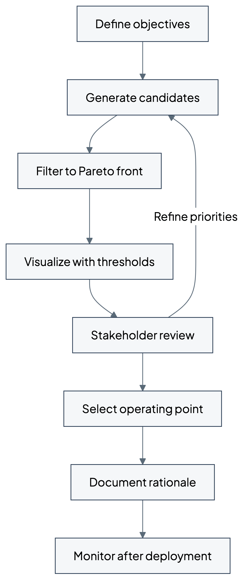
Because the choice reflects values, the record of it is part of the assurance evidence. The documentation should name the objectives and how each was measured, the method used to generate the frontier and its known blind spots (for example, that a weighted sum cannot reach non-convex regions), the full set of non-dominated candidates with their metrics, the thresholds and benchmarks marked on the plots, who took part in the decision, the selected point and the reasons it was preferred over its neighbors. The record should be revisited when priorities change or better generation methods become available, so that the choice can be refined rather than inherited.

Where multi-objective optimization sits in a learning system

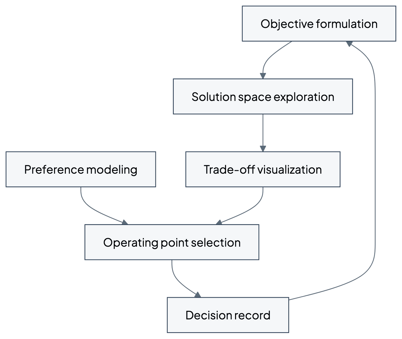
From a system perspective, multi-objective optimization for fairness touches five components:

• Objective formulation. Performance and each fairness criterion are modeled as separate, explicitly defined objectives rather than combined implicitly.
• Solution space exploration. Techniques generate a diverse set of Pareto optimal solutions rather than a single point.
• Trade-off visualization. The multi-dimensional trade-off space is represented in a way stakeholders can read.
• Preference modeling. Stakeholder priorities and value judgments are captured, whether as weights, bounds or reference points.
• Operating point selection. A decision process selects one solution from the front and records why.

This mapping shows that the approach changes the development process itself rather than adding fairness as an afterthought. Model selection and hyperparameter tuning, which normally optimize a single validation metric, become a search over a vector of metrics followed by a documented choice.

Source: validant.ai.

Intersectionality and many objectives

Why single-attribute objectives are not enough

Many multi-objective formulations optimize fairness for each protected attribute separately and so miss disparities at the intersections of attributes (Chapter 29). Buolamwini and Gebru (2018) showed how large such disparities can be. Evaluating three commercial gender classification systems on a new benchmark balanced by gender and skin type, they found darker-skinned females to be the most misclassified group, with error rates of up to 34.7 percent, while the maximum error rate for lighter-skinned males was 0.8 percent. They also found the two existing benchmarks they examined to be overwhelmingly composed of lighter-skinned subjects (79.6 percent for IJB-A and 86.2 percent for Adience). An evaluation by gender alone or by skin type alone would have obscured where the failures concentrated.

In a resume screening system, a conventional formulation might balance accuracy against gender fairness and racial fairness separately. An intersectional formulation adds objectives for each combination of gender and race, so that the system is assessed for Black women, Asian men and every other combination, not only for the aggregate categories. Fairness gerrymandering, in which a classifier appears fair on each attribute separately while violating fairness on structured subgroups, is the formal version of this risk (Kearns et al., 2018).

Intersectional fairness objectives

Foulds, Islam, Keya and Pan (2020) propose differential fairness, which bounds how much the probability of any outcome may differ between any two intersectional groups. A mechanism M is ε-differentially fair if, for every outcome y and every pair of intersectional groups s_i, s_j (tuples of all protected attribute values) with positive probability,

The definition is stated over a set of plausible data distributions θ; the display suppresses that conditioning. A single ε then summarizes the worst ratio across all intersections, which makes it a convenient single objective, or a constraint, to place alongside performance.

The curse of many objectives

Including intersections multiplies the objectives. With gender at two levels and race at four, there are 6 marginal groups but 8 intersectional cells and 28 pairwise gaps between cells. Adding an age band at three levels gives 9 marginal groups, 24 cells and 276 pairwise gaps. Even if the gaps are summarized per cell, the number of objectives grows with the product of the attribute levels.

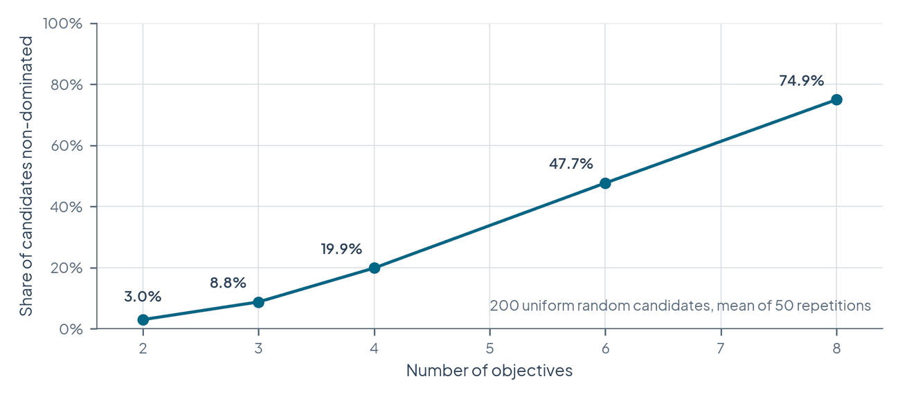
More objectives also weaken dominance as a filter. In a simulation for this chapter with 200 random candidate points drawn uniformly in objective space, averaged over 50 repetitions, the share of points that were non-dominated was 3.0 percent with two objectives, 8.8 percent with three, 19.9 percent with four, 47.7 percent with six and 74.9 percent with eight. With many objectives most candidates survive the Pareto filter, so the filter no longer narrows the choice and preference information is needed earlier. This is the motivation for many-objective algorithms such as NSGA-III, developed for problems with four or more objectives (Deb & Jain, 2014).

Source: validant.ai.

Requirements for intersectional multi-objective work

Addressing intersectionality in a multi-objective framework requires four things:

1. Including intersectional fairness objectives explicitly in the formulation, not only marginal ones.
2. Visualization techniques that communicate intersectional trade-offs to stakeholders, such as heatmaps of subgroup metrics.
3. Preference articulation methods that cope with higher-dimensional objective spaces, for example by fixing bounds on some objectives and trading off the rest.
4. Optimization methods that scale to many objectives without becoming computationally intractable.

Small intersectional cells add a statistical problem: their metrics are estimated from few cases and are noisy, so an apparent trade-off may be sampling variation (Chapters 41 and 43). Frontier points that differ only within the confidence intervals of a small subgroup's metric should not be treated as genuinely different.

A structured implementation method

The following method organizes multi-objective fairness work into four steps.

1. Trade-off analysis and objective definition. Name the performance metrics relevant to the application (accuracy, F1-score, AUC, or a cost-weighted error) and the fairness criteria to be satisfied (demographic parity, equal opportunity and others). Analyze potential conflicts through preliminary experiments or theory, for example the impossibility results of Chapter 19. Record every objective with a precise mathematical definition, the data on which it is evaluated and its direction.
2. Frontier exploration. Choose a generation method (see the table above). For linear scalarization, train one model per value of λ in a combined objective; for the ε-constraint method, optimize performance under a sequence of fairness bounds; for possibly non-convex fronts, add Chebyshev or boundary-intersection runs. Verify the Pareto optimality of the results by checking that no candidate is dominated.
3. Evaluation and visualization. Compute all performance, fairness and application-specific metrics for every candidate. Use two-dimensional plots for two-objective problems, parallel coordinate plots for higher-dimensional objective spaces and radar charts for comparing a few specific solutions. Annotate the plots with context such as baseline performance and legal or regulatory benchmarks.
4. Preference articulation and selection. For a priori articulation, encode stakeholder preferences as weights or bounds; for a posteriori articulation, present the front and support the choice with interactive tools; for interactive articulation, build a feedback loop that refines the search. Document the rationale and the value judgments it reflects.

A minimal sketch of a weighted-sum sweep follows; the metric functions stand for whatever performance and fairness measures step 1 defined.

def combined_objective(params, lam):

performance_loss = performance_loss_fn(params) # for example cross-entropy

fairness_loss = fairness_loss_fn(params) # for example squared DP gap

return (1 - lam) * performance_loss + lam * fairness_loss

candidates = []

for lam in [0.0, 0.05, 0.1, 0.2, 0.3, 0.5, 0.7, 0.9]:

params = train(combined_objective, lam, init=previous_params) # warm start

candidates.append(evaluate_all_metrics(params))

front = [c for c in candidates if not any(dominates(o, c) for o in candidates)]

These steps extend ordinary model selection and hyperparameter tuning rather than replacing them. They add analytical work, but they replace ad hoc adjustments and hidden trade-offs with an explicit, reviewable procedure.

Implementation challenges

Computational cost. Mapping a frontier means training many models. Useful remedies are warm-starting each run from the solution for a neighboring weight or bound; approximation methods such as evolutionary algorithms for large problems; adaptive sampling that spends computation on the regions of the front that matter, such as the neighborhood of a legal benchmark or of the knee; and transfer learning or fine-tuning, which adapts a trained model to a new trade-off point instead of training from scratch.

High-dimensional objective spaces. Several fairness criteria and intersectional subgroups create trade-off spaces that are hard to explore and to show. Remedies include analyzing correlations between objectives and reducing them to the most informative ones, for example with principal component analysis of the objective values; progressive exploration that starts with the primary objectives and adds others incrementally; visualization designed for many dimensions; and interactive tools that let stakeholders explore guided slices of the space.

Successful use requires computing capacity for exploring many solutions, expertise in both machine learning and multi-objective optimization, and sustained stakeholder engagement for selecting the operating point.

Evaluating a multi-objective result

Verifying Pareto optimality

• Dominance analysis. Confirm that no reported candidate is dominated by another candidate, including candidates from baseline methods.
• Local improvement tests. Perturb solutions (for example small changes of threshold or weights) and check that no local adjustment improves all objectives at once.
• Baseline comparison. Compare against unconstrained training and single-criterion methods to confirm that the multi-objective procedure actually widens the range of available trade-offs.
• Generalization. Recompute the objectives of the final candidates on held-out data. A front estimated on validation data can reorder on test data, and dominance relations that rest on differences within sampling error are not reliable (Chapter 41).
• Documentation. Record the verification results as evidence of the quality of the computed front.

The hypervolume indicator

The hypervolume indicator of a point set S with reference point r, for minimization, is the Lebesgue measure Λ of the region that S weakly dominates and r bounds (Guerreiro et al., 2022):

and the contribution of a point p is how much the measure shrinks when p is removed:

It was first proposed for assessing multi-objective optimizers (Zitzler & Thiele, 1999) and rewards closeness to the front, diversity and spread at the same time. Its distinguishing theoretical property is strict monotonicity with respect to set dominance: a set that dominates another always has a larger hypervolume (Guerreiro et al., 2022). In two dimensions it is computed by sorting the points; in general dimension, computing it and computing a single point's contribution are #P-hard problems (Guerreiro et al., 2022), which limits its use with many objectives. Its value depends on the reference point and on the scaling of the objectives, so comparisons are meaningful only with the same reference point and scaling.

In practice, the hypervolume serves four purposes: comparing a method's front with benchmark fronts, tracking convergence as more models are trained, quantifying how much a new method improves the available trade-offs, and using contributions to identify especially valuable solutions, such as the knee model D in the credit example.

Evaluating the decision process

The front exists to support a decision, so the process should be evaluated too. Structured assessments can establish whether the presented trade-offs answered stakeholders' needs, whether the visualizations were clear and useful, how much time and effort the selection took, and what stakeholders recommend changing next time. These evaluations belong within the organization's wider fairness assessment framework (Chapter 36).

Case study: lending with several fairness criteria

The following case comes from the source material and is a composite illustration; its figures are scenario values, not results from a real deployment.

Context. A financial institution builds a model that predicts default risk from credit history, income, employment stability and other financial indicators; the risk scores inform lending decisions. The risk management team wants accurate default prediction, compliance officers monitor fair lending, borrowers seek equitable access to credit, and business leaders focus on portfolio performance. In U.S. consumer credit, the Equal Credit Opportunity Act makes it unlawful for a creditor to discriminate against an applicant in any aspect of a credit transaction on the basis of race, color, religion, national origin, sex or marital status, or age (15 U.S.C. § 1691(a)). The statute does not prescribe demographic parity; the institution adopts the approval-rate gap as a monitoring metric, alongside equal opportunity for creditworthy applicants. Creditworthiness indicators are distributed differently across groups because of historical inequities, so the objectives conflict.

Problem analysis. Four challenges appear. First, an inherent trade-off: initial experiments suggest that strict demographic parity would reduce predictive accuracy considerably, by about 15 percent in the risk team's estimate, because it restricts the use of predictive features correlated with protected attributes. Second, competing fairness definitions: perfect demographic parity would require approving some higher-risk applications from certain groups, which can conflict with equal opportunity for truly low-risk applicants in all groups. Third, intersectional effects: the model looks reasonable for gender and race separately but shows significant disparities for specific combinations, such as younger women from certain racial backgrounds. Fourth, stakeholder tension: business leaders prioritize accuracy, compliance officers emphasize the approval-rate gap and borrower advocates press for equal opportunity, and not all can be satisfied to the fullest. Ad hoc tuning or a single criterion would hide these trade-offs.

Solution. The team defined three objectives: predictive performance measured by AUC (minimized as 1 − AUC), the difference in approval rates across racial groups, and the difference in true positive rates across racial groups. It trained models under a range of weight combinations for the three objectives,

and filtered the results to non-dominated models. (Because the AUC is not differentiable, training would use a smooth surrogate, Chapter 52; and because a weighted sum misses non-convex regions, adding ε-constraint runs at the compliance bounds would have been prudent.) It built interactive visualizations of the three-dimensional front, with two-dimensional projections such as accuracy against the approval-rate gap, annotated with the compliance team's internal thresholds and with business performance requirements. Selection was a posteriori: stakeholders reviewed operating points in a structured process and chose a model that kept 95 percent of the original predictive accuracy, brought the approval-rate gap below the internal threshold and kept the equal opportunity difference below 5 percent. The team then added objectives for key intersections, accepted the higher-dimensional search this required, and verified that the selected model met its fairness thresholds for both the main groups and the intersections. Trade-offs, design decisions and rationales were documented throughout.

Outcomes and lessons. The approach made the trade-offs between accuracy and each fairness criterion visible, produced a better balance than either unconstrained training or a single-criterion method, and turned a contentious disagreement into a collaborative decision over concrete options. Its costs were the computation needed to map the front, reduced by warm-starting, and the difficulty of explaining multi-dimensional trade-offs to non-technical stakeholders, addressed with carefully annotated visualizations. Three lessons generalize: model the objectives explicitly instead of combining them implicitly; generate and visualize a diverse set of non-dominated solutions before committing to a trade-off; and treat operating point selection as a structured stakeholder decision, since it reflects value judgments as much as technical facts.

Objective	Measure	Selection outcome
Predictive performance	1 − AUC	95 percent of original accuracy kept
Demographic parity	Approval-rate gap across racial groups	Below the internal threshold
Equal opportunity	TPR gap across racial groups	Below 5 percent
Intersectional fairness	Metrics for key intersections	Thresholds met for groups and intersections

Source: illustrative case from the source materials, restated by validant.ai.

Competing interpretations and limitations

Efficiency is not fairness

Pareto optimality is an efficiency notion borrowed from economics. It rules out models that waste performance or fairness, but every point on the front, including the most unequal one, is efficient. A front can be computed perfectly and the choice from it can still be indefensible. Multi-objective methods structure the normative decision; they do not make it.

Objectives or constraints?

Some requirements are not up for trade. A legal prohibition or a binding policy bound belongs in the feasible set as a constraint, not on an axis to be weighed against accuracy. Treating a legal floor as one more objective invites the impression that it can be bought out with enough accuracy. The ε-constraint method expresses this naturally; a weighted sum does not.

The frontier depends on its method

As the credit example shows, the generation method determines which compromises appear. A team that sweeps a penalty weight and reports the resulting curve may present an incomplete front without knowing it (Wei & Niethammer, 2022). Conversely, under convexity the weighted sum is complete (Martinez et al., 2020). The method and its blind spots should be stated with the results.

Where to place the trade-off

Kleinberg et al. (2018) argue that fairness preferences should change how predictions are used rather than the estimator itself, which favors exploring the trade-off over decision rules. Others favor building fairness into training, especially where group-specific decision rules are legally constrained or where representations themselves carry harm (Chapter 53). Which placement is preferable depends on the legal regime, the model class and the criterion.

Randomization and individual treatment

Randomized mixtures can dominate deterministic models, as the worked example shows, and reductions methods return them by design (Agarwal et al., 2018). Yet a policy under which identical applicants may receive different decisions by chance can conflict with individual fairness, with expectations of consistency and with the ability to explain a decision to the person affected.

Estimated, not true, frontiers

Every empirical front is estimated from finite data. Differences between neighboring points may be within sampling error, particularly for subgroup metrics, and the front can shift under distribution change after deployment (Chapter 34). A front should carry uncertainty estimates where possible and be recomputed when the data change.

Common questions

How does multi-objective optimization differ from fairness regularization, and when should each be used? Both handle the fairness-performance trade-off, but they frame it differently. Regularization adds fairness as a penalty to a primarily performance-focused objective, with a hand-tuned weight setting the balance; the trade-off is navigated implicitly through that weight, without mapping the whole space. Multi-objective optimization models the objectives separately and explores the frontier systematically, so the choice rests on knowledge of the available options. Regularization suits cases that need a simpler implementation with lower computational cost and where the team already has a sound sense of the appropriate balance.

Multi-objective optimization suits cases that require a thorough understanding of the trade-offs, where stakeholders with different priorities must reach agreement, or where more than two objectives must be balanced, such as several fairness criteria alongside performance. It costs more computation but offers more transparency and a more principled path through complex trade-offs, which is most valuable in high-stakes applications. A penalized loss with a deliberate sweep of its weight is itself a simple multi-objective method, subject to the limits of linear scalarization.

How can many fairness criteria across several protected attributes and their intersections be handled? Several approaches help keep the problem tractable and meaningful. First, analyze correlations between fairness metrics: some are highly correlated, so a few representative metrics can stand for related concerns. Second, use progressive preference articulation: compute the front for the primary objectives first, then add further criteria as constraints, which lowers the dimension of each phase. Third, use hierarchical approaches that group related objectives, for example by protected attribute or by type of fairness definition, and optimize within groups before balancing across them. Fourth, apply dimensionality reduction such as principal component analysis to the objective values to identify the dominant trade-off directions. Fifth, use algorithms designed for many objectives, such as NSGA-III or other reference-point methods (Deb & Jain, 2014). Sixth, build visualizations suited to high dimensions, such as heatmaps of intersectional metrics or interactive tools that show selected slices of the objective space. Start with a reduced set of objectives to establish baseline trade-offs and add criteria as understanding and computational capacity allow.

Is a model chosen from the frontier automatically fair? No. It is efficient with respect to the objectives that were measured, on the data that were used. It may still rely on a biased label, use proxies for the protected attribute, fail for an unmeasured subgroup or drift after deployment. The frontier is one piece of evidence within a wider assessment (Chapter 36).

How many models need to be trained? Enough to locate the regions that matter: the extremes, the knee and the neighborhood of any legal or policy bound. A coarse sweep followed by refinement where the front bends or where points are sparse, in the spirit of adaptive weighting (Kim & de Weck, 2005), is usually more efficient than a fine uniform grid. Warm-starting keeps the cost down.

Can stakeholders legitimately choose a dominated model? Only if the objectives that make it dominated are incomplete. If a dominated model is preferred for a reason, such as simplicity, interpretability or a lower cost of operation, that reason is an unmeasured objective and should be added to the formulation and documented. Otherwise a dominated model is never the right choice.

Should the frontier be shown to non-technical stakeholders? Yes, in a form they can read. Start with two-objective plots, annotate them with baselines and benchmarks, and show the concrete consequences of moving between points, for example how many additional applicants would be approved per thousand. Teams new to the approach should begin with a simple two-objective problem, such as accuracy against demographic parity, before moving to several criteria, and use visualization to build intuition about the trade-off space and stakeholders' confidence in navigating it explicitly.

Conclusions

Fairness-aware learning is a multi-objective problem, and treating it as one makes the hidden choices of single-objective training explicit. The tension between fairness and performance is real wherever base rates differ and the fairness criterion changes the optimal rule, but its size varies and must be measured; a steep frontier is as much a finding about the data as a menu of compromises.

Pareto optimality gives the analysis its discipline: dominated models are excluded, and the remaining choice is narrowed to genuine trade-offs. The method used to compute the frontier is not neutral. Weighted sums, which include ordinary fairness penalties, can only find points on the convex hull and spread unevenly; the ε-constraint method, Chebyshev scalarization, boundary-intersection methods and evolutionary algorithms can reach the rest, and randomized mixtures can fill in the hull at a cost to individual consistency.

Selecting an operating point is a value judgment that belongs to identified stakeholders, informed by legal benchmarks, and recorded with its reasons. For assurance purposes, the evidence of record is the frontier, the method that produced it, the selection rule and the rationale, not the chosen model alone. With intersectional subgroups the number of objectives grows quickly, dominance loses its power to narrow the choice, and preferences and structure must enter earlier.

Open questions

• Which selection rule, if any, should serve as a default for choosing a point on a fairness frontier, and how should the choice depend on domain and legal regime?
• How can fairness frontiers be estimated with honest uncertainty, especially for small intersectional subgroups, and how should dominance be tested statistically?
• When does training-time multi-objective optimization add value beyond exploring the trade-off over decision thresholds of a single well-calibrated predictor?
• How do frontiers computed before deployment change under distribution shift, and how often must they be recomputed?
• How can many-objective fairness problems be presented to stakeholders so that their choices reflect informed preferences rather than the artifacts of a visualization?
• Under what conditions are randomized classifiers acceptable in regulated decisions about individuals?

References

• Agarwal, A., Beygelzimer, A., Dudík, M., Langford, J., & Wallach, H. (2018). A reductions approach to fair classification. In Proceedings of the 35th International Conference on Machine Learning (Proceedings of Machine Learning Research, Vol. 80, pp. 60 - 69). https://proceedings.mlr.press/v80/agarwal18a.html
• Agarwal, A., Dudík, M., & Wu, Z. S. (2019). Fair regression: Quantitative definitions and reduction-based algorithms. In Proceedings of the 36th International Conference on Machine Learning (Proceedings of Machine Learning Research, Vol. 97, pp. 120 - 129). https://proceedings.mlr.press/v97/agarwal19d.html
• Buolamwini, J., & Gebru, T. (2018). Gender shades: Intersectional accuracy disparities in commercial gender classification. In Proceedings of the 1st Conference on Fairness, Accountability and Transparency (Proceedings of Machine Learning Research, Vol. 81, pp. 77 - 91). https://proceedings.mlr.press/v81/buolamwini18a.html
• Corbett-Davies, S., Pierson, E., Feller, A., Goel, S., & Huq, A. (2017). Algorithmic decision making and the cost of fairness. In Proceedings of the 23rd ACM SIGKDD International Conference on Knowledge Discovery and Data Mining (pp. 797 - 806). ACM. https://doi.org/10.1145/3097983.3098095
• Das, I., & Dennis, J. E. (1997). A closer look at drawbacks of minimizing weighted sums of objectives for Pareto set generation in multicriteria optimization problems. Structural Optimization, 14(1), 63 - 69. https://doi.org/10.1007/BF01197559
• Das, I., & Dennis, J. E. (1998). Normal-boundary intersection: A new method for generating the Pareto surface in nonlinear multicriteria optimization problems. SIAM Journal on Optimization, 8(3), 631 - 657. https://doi.org/10.1137/S1052623496307510
• Deb, K., & Jain, H. (2014). An evolutionary many-objective optimization algorithm using reference-point-based nondominated sorting approach, Part I: Solving problems with box constraints. IEEE Transactions on Evolutionary Computation, 18(4), 577 - 601. https://doi.org/10.1109/TEVC.2013.2281535
• Deb, K., Pratap, A., Agarwal, S., & Meyarivan, T. (2002). A fast and elitist multiobjective genetic algorithm: NSGA-II. IEEE Transactions on Evolutionary Computation, 6(2), 182 - 197. https://doi.org/10.1109/4235.996017
• Emmerich, M. T. M., & Deutz, A. H. (2018). A tutorial on multiobjective optimization: Fundamentals and evolutionary methods. Natural Computing, 17(3), 585 - 609. https://doi.org/10.1007/s11047-018-9685-y
• Equal Credit Opportunity Act, 15 U.S.C. § 1691. https://www.law.cornell.edu/uscode/text/15/1691
• Foulds, J. R., Islam, R., Keya, K. N., & Pan, S. (2020). An intersectional definition of fairness. In 2020 IEEE 36th International Conference on Data Engineering (ICDE) (pp. 1918 - 1921). IEEE. https://doi.org/10.1109/ICDE48307.2020.00203
• Guerreiro, A. P., Fonseca, C. M., & Paquete, L. (2022). The hypervolume indicator: Computational problems and algorithms. ACM Computing Surveys, 54(6), 1 - 42. https://doi.org/10.1145/3453474
• Kearns, M., Neel, S., Roth, A., & Wu, Z. S. (2018). Preventing fairness gerrymandering: Auditing and learning for subgroup fairness. In Proceedings of the 35th International Conference on Machine Learning (Proceedings of Machine Learning Research, Vol. 80, pp. 2564 - 2572). https://proceedings.mlr.press/v80/kearns18a.html
• Kim, I. Y., & de Weck, O. L. (2005). Adaptive weighted-sum method for bi-objective optimization: Pareto front generation. Structural and Multidisciplinary Optimization, 29(2), 149 - 158. https://doi.org/10.1007/s00158-004-0465-1
• Kleinberg, J., Ludwig, J., Mullainathan, S., & Rambachan, A. (2018). Algorithmic fairness. AEA Papers and Proceedings, 108, 22 - 27. https://doi.org/10.1257/pandp.20181018
• Martinez, N., Bertran, M., & Sapiro, G. (2020). Minimax Pareto fairness: A multi objective perspective. In Proceedings of the 37th International Conference on Machine Learning (Proceedings of Machine Learning Research, Vol. 119, pp. 6755 - 6764). https://proceedings.mlr.press/v119/martinez20a.html
• Uniform Guidelines on Employee Selection Procedures (1978), 29 C.F.R. § 1607.4, Information on impact. https://www.law.cornell.edu/cfr/text/29/1607.4
• Valdivia, A., Sánchez-Monedero, J., & Casillas, J. (2021). How fair can we go in machine learning? Assessing the boundaries of accuracy and fairness. International Journal of Intelligent Systems, 36(4), 1619 - 1643. https://doi.org/10.1002/int.22354
• Wei, S., & Niethammer, M. (2022). The fairness-accuracy Pareto front. Statistical Analysis and Data Mining: The ASA Data Science Journal, 15(3), 287 - 302. https://doi.org/10.1002/sam.11560
• Zafar, M. B., Valera, I., Gomez Rodriguez, M., & Gummadi, K. P. (2017). Fairness constraints: Mechanisms for fair classification. In Proceedings of the 20th International Conference on Artificial Intelligence and Statistics (Proceedings of Machine Learning Research, Vol. 54, pp. 962 - 970). https://proceedings.mlr.press/v54/zafar17a.html
• Zafar, M. B., Valera, I., Gomez-Rodriguez, M., & Gummadi, K. P. (2019). Fairness constraints: A flexible approach for fair classification. Journal of Machine Learning Research, 20(75), 1 - 42. https://jmlr.org/papers/v20/18-262.html
• Zitzler, E., & Thiele, L. (1999). Multiobjective evolutionary algorithms: A comparative case study and the strength Pareto approach. IEEE Transactions on Evolutionary Computation, 3(4), 257 - 271. https://doi.org/10.1109/4235.797969